The extended memory hierarchy

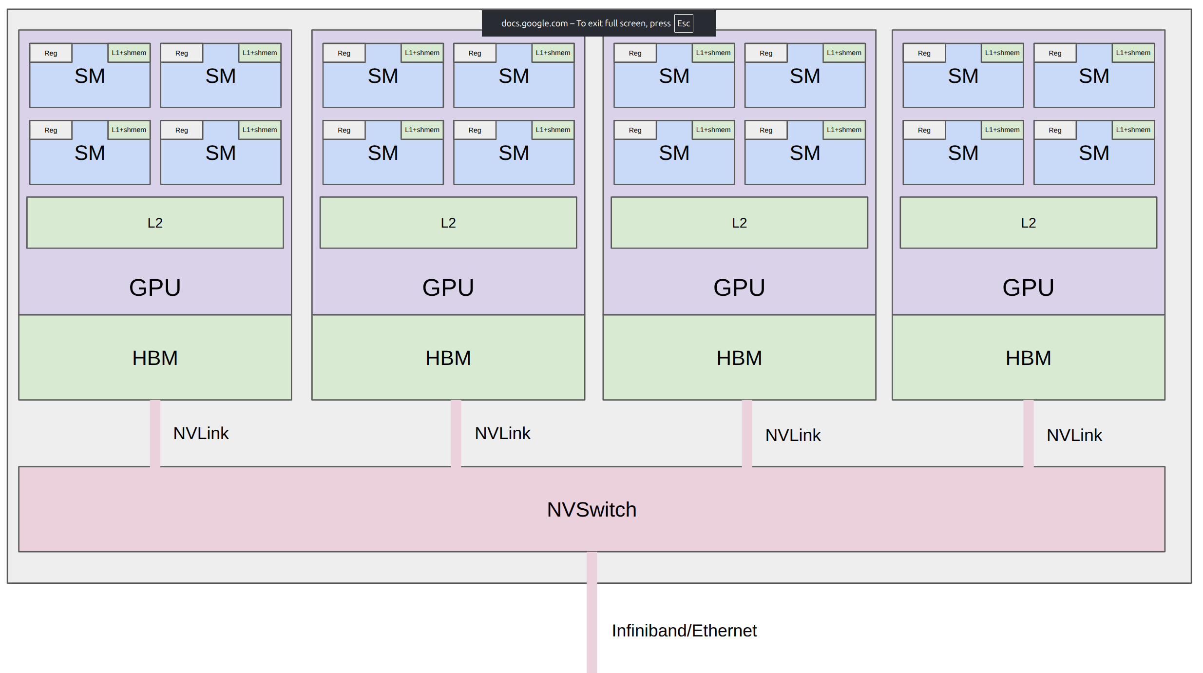From one GPU to many: GPUs in a node linked by NVLink/NVSwitch, nodes linked by InfiniBand/Ethernet. Source: CS336 Lecture 7.

Everything is one hierarchy now, fastest to slowest:

You go multi-GPU for two reasons: (1) the model (params + gradients + optimizer state + activations) doesn't fit in one GPU's HBM (a 1T-param model won't fit in a B200's 192 GB), or (2) you want more FLOPs to train faster. It's easy to use many GPUs; hard to use them effectively.

The vocabulary of distributed programming

A rank is a device (GPU); world size is the number of devices. Source: CS336 Lecture 7.

Collective operations are 1980s parallel-programming primitives that specify a whole communication pattern across devices, rather than point-to-point messaging — easier to write and faster, since the system can optimize the pattern. The foundations (broadcast, scatter, gather, reduce) are warm-ups; the workhorses are all-gather, reduce-scatter, all-reduce; all-to-all is for MoEs.

Worked examples on 4 ranks (input rows are [0,1,2,3]+rank):

# reduce-scatter: reduce each column, scatter to ranks
ranks in:  [0 1 2 3] [1 2 3 4] [2 3 4 5] [3 4 5 6]
ranks out: [6]       [10]      [14]      [18]        # col sums, one per rank

# all-reduce: reduce, then replicate everywhere
ranks out: [6 10 14 18]  (on every rank)

# all-to-all (the position = destination rank) ≈ transpose
in:  [0 1 2 3] [4 5 6 7] [8 9 10 11] [12 13 14 15]
out: [0 4 8 12] [1 5 9 13] [2 6 10 14] [3 7 11 15]

The hardware underneath

Classically: GPUs in a node talk over a PCIe bus; across nodes, over Ethernet (slow). In a real data center:

• 8 GPUs / node connected by NVLink to an NVSwitch — NVLink 5.0 gives ~1.8 TB/s (vs 8 TB/s for HBM, so ~4× slower than local memory, but very fast between devices). From the programmer's view, NVSwitch makes any GPU reachable from any other.
• ~256 nodes / pod connected by InfiniBand (~0.05 TB/s), via PCIe → HCA/NIC → cable.
• pods → cluster over Ethernet, which routes through the CPU (slowest).

At the bottom, NCCL ("nickel," NVIDIA Collective Communications Library) turns a collective like all-reduce into actual packets: it detects the hardware topology, optimizes the path between GPUs, and launches communication kernels (everything on a GPU is a kernel — including comms).

In PyTorch: torch.distributed

torch.distributed wraps the collectives with backends per hardware (gloo for CPU, nccl for GPU). You spawn a function across world_size processes, each with its own rank:

def setup(rank, world_size):
    os.environ["MASTER_ADDR"] = "localhost"   # for coordination only; data goes via NCCL
    os.environ["MASTER_PORT"] = "15623"
    dist.init_process_group("nccl", rank=rank, world_size=world_size)

dist.barrier()                                  # wait for all processes to reach here
dist.all_reduce(tensor=data, op=dist.ReduceOp.SUM)  # modifies data in place
dist.reduce_scatter_tensor(output=out, input=inp, op=dist.ReduceOp.SUM)
dist.all_gather_into_tensor(output_tensor=out, input_tensor=inp)

Two kinds of asynchrony stack here — CUDA kernels are async, and the processes run independently — so you use torch.cuda.synchronize() (wait for kernels) and dist.barrier() (wait for processes). With async_op=True a collective returns immediately, letting you overlap communication with computation (e.g. prefetch the next batch while gradients reduce).

Benchmarking collective bandwidth

Analogous to MFU, measure effective bandwidth = bytes that need to be sent ÷ time. For all-reduce, each rank does world_size − 1 add-steps, ×2 for send+receive:

sent_bytes     = size_bytes * 2 * (world_size - 1)
total_duration = world_size * duration
bandwidth      = sent_bytes / total_duration      # ≈ 400 GB/s in the demo

As world size grows, (world_size−1)/world_size → 1, so effective bandwidth ≈ 2·size/duration — independent of world size and of topology (ring vs tree; NCCL decides). Reduce-scatter has no ×2, so all-reduce moves twice the data in twice the time → the same bandwidth.

Data parallelism — cut the batch

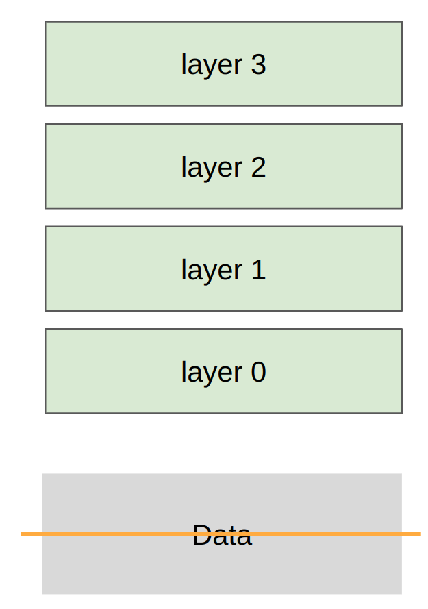Each rank holds all parameters but processes a different slice of the batch. Source: CS336 Lecture 7.

Split the batch rows across ranks; every rank keeps the full model and its own optimizer state, trains on its local batch, then synchronizes gradients. The only difference from single-GPU training is one line after backward():

for param in params:                 # forward + backward on the LOCAL batch, then:
    dist.all_reduce(tensor=param.grad, op=dist.ReduceOp.AVG)  # ← the whole trick
optimizer.step()

After the all-reduce every rank has identical (averaged) gradients, so parameters stay in lockstep — each rank updates as if it had seen the whole batch. Losses and initial gradients differ across ranks; the all-reduce makes gradients (and thus params) the same. It's elegant and model-agnostic (DDP doesn't care what the forward pass is). The limitation: every rank must hold all parameters in memory — FSDP/ZeRO (next lecture) fixes that with all-gather + reduce-scatter. (This is "DDP", distributed data parallel.)

Tensor parallelism — cut the width

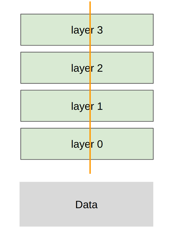Each rank holds a column-slice of every layer's weight matrix and all the data. Source: CS336 Lecture 7.

Now cut the other way: each layer's weight matrix is split (here by columns → "column tensor parallel"), so each rank owns a num_dim × local_num_dim slice and all ranks see all the data. Per layer:

for layer in range(num_layers):
    x = x @ params[layer]          # only a SLICE of the weights → partial activations
    x = F.gelu(x)                  # elementwise, so fine on the slice
    dist.all_gather(activations, x)  # collect every rank's slice
    x = torch.cat(activations, dim=1)  # reassemble full batch_size × num_dim

You exploit that a matmul splits into smaller matmuls done on different ranks, then gathered. On the backward pass the dual happens: reduce-scatter the gradients (forward all-gathers, backward reduce-scatters). Unlike DDP, you must muck with the model itself — and you move a lot of data (full activations every layer), so this only makes sense over fast interconnects.

Pipeline parallelism — cut the depth

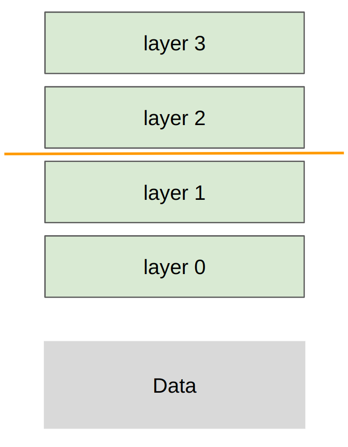Each rank owns a contiguous subset of layers; activations flow rank→rank. Source: CS336 Lecture 7.

Split by layers: rank 0 holds the first layers, rank 1 the next, etc. Activations are passed with point-to-point send/recv:

for x in micro_batches:
    if rank - 1 >= 0: dist.recv(tensor=x, src=rank - 1)   # from previous rank
    for param in local_params:                          # my layers only
        x = F.gelu(x @ param)
    if rank + 1 < world_size: dist.send(tensor=x, dst=rank + 1)  # to next rank

Choosing (and combining) strategies

Real runs combine them — typically tensor parallel within a node (NVLink), data/FSDP across nodes, and pipeline parallel when needed. Watch for the critical batch size: past it, scaling data parallelism stops helping, so you switch to tensor/pipeline. Other axes exist — sequence parallelism (split the sequence, for attention) and expert parallelism (split experts for MoE, the all-to-all use case). On JAX/TPU you can instead just declare the model and a sharding strategy and let the compiler insert the collectives (e.g. Levanter) — convenient, but less instructive than building from primitives.

Golden rules & takeaways

• Same theme, bigger scale: compute is far from data; orchestrate to minimize transfer. Single-GPU it was fusion/tiling; multi-GPU it's replication/sharding over collectives.
• Learn the workhorses: all-gather, reduce-scatter, all-reduce — and remember all-reduce = reduce-scatter + all-gather.
• Topology is a hierarchy: NVLink/NVSwitch (fast, in-node) → InfiniBand (pod) → Ethernet (cluster); RDMA bypasses the CPU. NCCL handles the routing.
• Data parallelism is a one-line change (all-reduce the gradients) but needs every rank to hold the full model — FSDP/ZeRO relaxes that.
• Tensor parallelism moves activations every layer → needs fast interconnects; pipeline parallelism tolerates slow links but must fight bubbles with micro-batches.
• Pick by hardware, and combine: tensor within a node, data/FSDP + pipeline across nodes. The "recompute vs store-in-memory vs store-on-another-GPU-and-communicate" trade-off is the same idea recurring.

Next: a deeper dive on parallelism — FSDP and ZeRO.

References

Primary source is the lecture (executable lecture_07.py). Key works & tools:

1. Collective operations (overview)
2. PyTorch — torch.distributed · NCCL performance docs
3. Shoeybi et al. (2019) — Megatron-LM (tensor parallelism)
4. Huang et al. (2018) — GPipe (pipeline parallelism)
5. Rajbhandari et al. (2019) — ZeRO (sharded data parallelism)
6. Levanter — JAX, declarative sharding