Writing Triton kernels (and measuring first)
A hands-on continuation of the GPU lecture: dive into the code. The discipline is benchmark and profile before you optimize; the tool is Triton, where you think in thread blocks. We build up from element-wise GeLU to a tiled matmul — everything you need to implement FlashAttention.
Recap: the hardware and its hierarchy
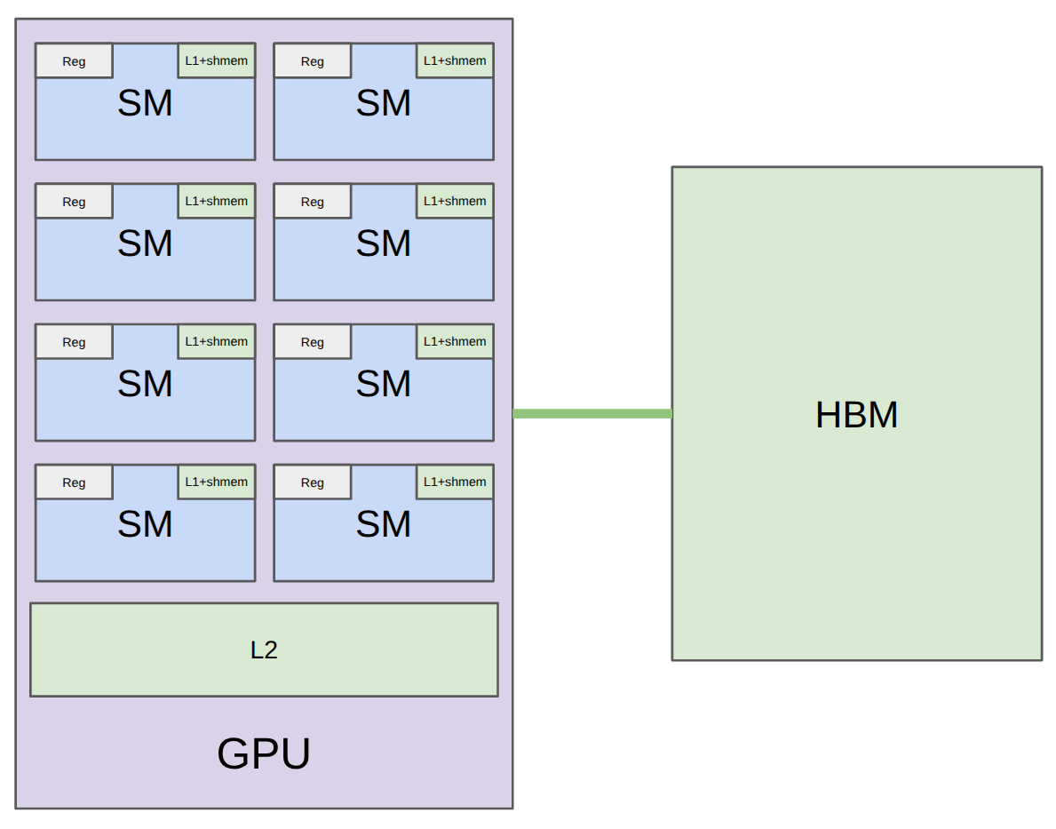 A GPU: ~100–200 SMs, each with registers + L1/shared memory; a chip-wide L2 cache; and large, slow HBM. Source: CS336 Lecture 6.
Across generations the SM count and on-chip memory barely move; HBM size and bandwidth are what grow. Sizes and bandwidths are inversely correlated — registers are tiny and blazing fast, HBM is huge and slow (though 8 TB/s isn't slow in absolute terms).
| Accelerator | A100 | H100 | B200 |
|---|---|---|---|
| # SMs | 108 | 132 | 148 |
| Registers / SM | 256 KB | 256 KB | 256 KB |
| L1 + shared / SM | 192 KB | 256 KB | 256 KB |
| L2 cache | 40 MB | 50 MB | 96–126 MB |
| HBM size | 80 GB | 80 GB | 192 GB |
| Register bandwidth | ~116 TB/s | ~401 TB/s | ~447 TB/s |
| L1 / shared bandwidth | ~19 TB/s | ~33 TB/s | ~19 TB/s |
| L2 bandwidth | ~5–8 TB/s | ~12 TB/s | ~9 TB/s |
| HBM bandwidth | 2 TB/s | 3.35 TB/s | 8 TB/s |
B200s also add tensor memory (TMEM) for tensor cores, sitting between registers and shared memory — invisible to the programmer.
The programming model: thread → block → grid
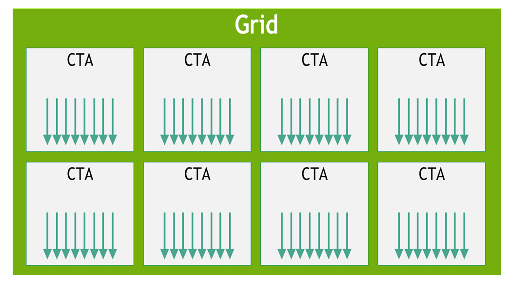 A grid of thread blocks (CTAs), each a group of threads. Launching a kernel launches a whole grid to run in parallel. Source: NVIDIA PTX docs.
- Thread
- Executes code on a small piece of the data.
- Thread block (CTA)
- A group of threads — and the reason blocks exist is shared memory.
- Grid
- The collection of thread blocks.
For element-wise ops (e.g. GeLU), plain threads suffice — one thread per element. But softmax and matmul need threads to communicate. You could communicate through HBM, but it's far too slow, so you use shared memory (local to an SM). A thread block is exactly "a set of threads that share one SM's shared memory," so a block is scheduled on a single SM: it reads from HBM, does work communicating via shared memory, and writes back. Triton makes you think natively in thread blocks — which turns out to be the sweet spot.
Where the model meets the hardware (5 considerations)
The programming model gives you correctness for free. Performance, though, is acutely sensitive to hardware details the model hides.
Warps
Within a block, threads are grouped into warps of 32 that execute the same instruction in lockstep. Control divergence — an if/else where threads disagree — serializes the two branches (bad). But the SM runs many resident warps and switches between them at zero cost, so when one warp blocks on a slow HBM read, another runs — hiding latency.
(Warp) occupancy
Each thread can use ≤ 255 registers, and an SM has a fixed register pool — so more registers per thread means fewer threads resident (lower occupancy). Low occupancy isn't necessarily bad (thread coarsening: fatten each thread to do more work). A worked example:
threads/block = 128,  registers/thread = 160   # what we want
max_registers/SM = 65536,  max_warps/SM = 64   # hardware limit

registers/block = 128 × 160 = 20480
blocks/SM       = 65536 // 20480 = 3           # limited by registers
warps           = 3 × 128 / 32 = 12
occupancy       = 12 / 64 = 18%          # register pressure caps us
Bank conflicts (shared memory)
Shared memory is split into 32 banks, each 4 bytes wide. Per cycle a bank serves one thread; if multiple threads hit the same bank, the accesses serialize. Worst case: 32 threads reading one column of a row-major matrix → a 32-way bank conflict. This is unavoidable in matmul (you read rows of A and columns of B). The fix is swizzling — rearranging shared memory (e.g. row XOR col) to spread accesses across banks.
Memory coalescing (HBM)
When a warp's 32 threads read HBM, accesses combine into 128-byte cache-line transactions. Full coalescing = all 32 threads hit the same cache line (32 × 4 bytes = 128). Strided/column access wastes most of each fetched line. (Bank conflicts are about shared memory; coalescing is about HBM — similar feel, different constraint.)
Block occupancy & wave quantization
 Blocks are scheduled onto SMs in waves. Source: NVIDIA developer blog.
A B200 has 148 SMs; launch 160 blocks and the first wave runs 148, the second runs just 12 — leaving most SMs idle (wave quantization). Fix: make the number of thread blocks divide the SM count.
Benchmark, then profile — always
The recipe for success: (1) benchmark and profile, (2) make a change, (3) benchmark and profile again. Measure where the bottlenecks are before writing any kernel.
Benchmarking — end-to-end wall time
It only gives total time (not where it's spent), but it's what you ultimately care about and shows scaling. The gotchas: warm up first (skip lazy-compilation cost), time multiple trials (variance), and use CUDA events with a synchronize (the GPU runs async, so naive CPU timers report impossibly fast).
for _ in range(num_warmups): run()
torch.cuda.synchronize()                 # wait for warmup to finish
for trial in range(num_trials):
    start, end = torch.cuda.Event(enable_timing=True), torch.cuda.Event(enable_timing=True)
    start.record(); run(); end.record()
    torch.cuda.synchronize()             # CRUCIAL: wait for the GPU
    times.append(start.elapsed_time(end))
Scaling matmul across dimensions reveals a key fact: time is roughly constant for small matrices, then grows cubically — because GPUs are built for large matmuls and a tiny one wildly underutilizes them.
Profiling — where time goes & what's under the hood
PyTorch has a built-in profiler (the assignment uses Nsight for more detail). Beyond timing, it reveals what your high-level code actually does. Profiling a + b shows a single CUDA functor add kernel; profiling a @ b shows a long-named kernel like:
cutlass3x_sm100_simt_sgemm_f32_..._64x64x16_...- cutlass
- NVIDIA's CUDA linear-algebra library
- sm100
- the Blackwell (B200) architecture
- f32
- float32
- 64×64×16
- the tile shape
Crucially, different tensor dimensions invoke different kernels (a 128×128 matmul picks a 32×32×16 tile vs 64×64×16 for larger) — the high-level @ hides a lot.
Case study: three GeLUs
Three implementations that compute the same thing with wildly different speed: a naive PyTorch expression, the built-in F.gelu, and torch.compile(naive). The built-in and compiled versions are far faster. The profiler explains why:
| Version | Kernels | HBM traffic |
|---|---|---|
| Naive PyTorch | many (one per primitive: mul, add, tanh, …) | read+write to HBM between every op (no fusion) |
| Built-in F.gelu | one hand-written CUDA kernel | one read, one write |
| torch.compile | one fused Triton kernel | one read, one write |
The naive version's computation graph realizes each primitive as a separate kernel, each round-tripping to HBM. Fusion (built-in or compiled) collapses them into one kernel: read once, compute in the SM, write once. The compiler literally emits a Triton kernel — a nice segue.
Think in thread blocks
CUDA vs Triton
| CUDA (NVIDIA) | Triton (OpenAI) | |
|---|---|---|
| You specify | what each thread does | what each thread block does |
| Pro | fine-grained control | handles shared memory / sync for you |
| Con | must manage sync & shared memory by hand | less control at the bleeding edge |
The Triton mental model for every kernel: load data into shared memory → operate on it (fuse!) → write back to HBM. It sits between PyTorch's giant-matrix view and CUDA's per-element view.
Example 1 · GeLU (element-wise)
The host code allocates the output, splits the data into blocks, and launches one program per block:
y = torch.empty_like(x)
BLOCK_SIZE = 1024                                # threads per block
num_blocks = triton.cdiv(x.numel(), BLOCK_SIZE)
triton_gelu_kernel[(num_blocks,)](x, y, x.numel(), BLOCK_SIZE=BLOCK_SIZE)
@triton.jit
def triton_gelu_kernel(x_ptr, y_ptr, num_elements, BLOCK_SIZE: tl.constexpr):
pid = tl.program_id(axis=0) # which block am I?
offsets = pid * BLOCK_SIZE + tl.arange(0, BLOCK_SIZE)
mask = offsets < num_elements # don't run past the end
x = tl.load(x_ptr + offsets, mask=mask) # read from HBM
a = 0.79788456 * (x + 0.044715 * x*x*x)
tanh = (tl.exp(2*a) - 1) / (tl.exp(2*a) + 1)
y = 0.5 * x * (1 + tanh)
tl.store(y_ptr + offsets, y, mask=mask) # write to HBMNote the shift in mindset: x_ptr/y_ptr are pointers (integers, addresses), there's no return value (you explicitly load and store), and a mask guards the final partial block. The body otherwise reads like normal PyTorch on a vector. Every kernel follows this shape: wake up → find my indices → load → compute → store.
Triton compiles down to PTX (GPU assembly). In it: ld.global/st.global are HBM reads/writes; %ctaid.x is the block index and %tid.x the thread index; %r*/%f* are integer/float registers. You'll also see one thread processing 8 elements — the compiler applied thread coarsening on its own. The PTX is one piece of code, compiled once, run by every thread, distinguished only by its (ctaid, tid). (When a thread hits a load that blocks on HBM, the warp scheduler swaps in another warp — that's the latency hiding from earlier.)
Example 2 · Softmax (reduction, row fits in a block)
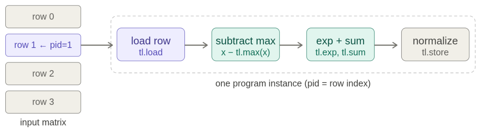 Softmax is row-wise, not element-wise: make each row a block. Blocks don't share memory, which is fine since rows are independent. Source: CS336 Lecture 6.
The naive PyTorch softmax (max → subtract → exp → sum → divide) costs 5MN + M reads and 3MN + 2M writes, where in principle MN/MN suffices — a ~4× waste, because each step is a separate kernel round-tripping through HBM. The Triton kernel does it in one pass; since a whole row fits in one block, the body is essentially the naive code:
@triton.jit
def triton_softmax_kernel(x_ptr, y_ptr, x_row_stride, y_row_stride, num_cols, BLOCK_SIZE: tl.constexpr):
    row = tl.program_id(0)                       # one block per row
    col = tl.arange(0, BLOCK_SIZE)
    x = tl.load(x_ptr + row*x_row_stride + col,
               mask=col < num_cols, other=float("-inf"))  # -inf = a 0 for softmax
    x = x - tl.max(x, axis=0)
    num = tl.exp(x)
    y = num / tl.sum(num, axis=0)
    tl.store(y_ptr + row*y_row_stride + col, y, mask=col < num_cols)
If a whole row fits in a block, Triton lets you write near-PyTorch code; the reduction happens inside the block automatically.
Example 3 · Row sum (reduction, row doesn't fit → baby tiling)
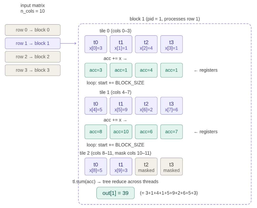 When a row (say 4096 cols) exceeds the block size (1024): break it into tiles, accumulate per-thread across tiles, then reduce. Source: CS336 Lecture 6.
Each block still owns one row, but now loops over tiles, keeping a per-thread accumulator, then reduces to a scalar:
@triton.jit
def row_sum_kernel(x_ptr, out_ptr, N, BLOCK_SIZE: tl.constexpr):
    row = tl.program_id(0)
    acc = tl.zeros([BLOCK_SIZE], dtype=tl.float32)   # per-thread accumulator
    for start in range(0, N, BLOCK_SIZE):           # loop over tiles
        cols = start + tl.arange(0, BLOCK_SIZE)
        x = tl.load(x_ptr + row*N + cols, mask=cols < N, other=0.0)
        acc += x
    result = tl.sum(acc, axis=0)                  # final reduction → scalar
tl.store(out_ptr + row, result)In the GeLU example the row was split into blocks processed independently. Here the block is the whole row, and the tiles are chunks that one block processes in a loop. This is where Triton stops looking like PyTorch — not everything fits in shared memory, so you iterate. The accumulator lives in registers or (if big) shared memory; Triton decides.
Example 4 · Matmul + ReLU (real tiling)
Three approaches, building to tiling:
| Approach | HBM reads | Arithmetic intensity | Problem |
|---|---|---|---|
| Naive (per output element, loop k) | O(MKN) | O(1) | massive redundant reads |
| Idealized (all of A, B in shared) | O(MK + KN) | O(N) | A, B don't fit in shared memory |
| Tiling | O(MKN / T) | O(tile size) | the practical winner |
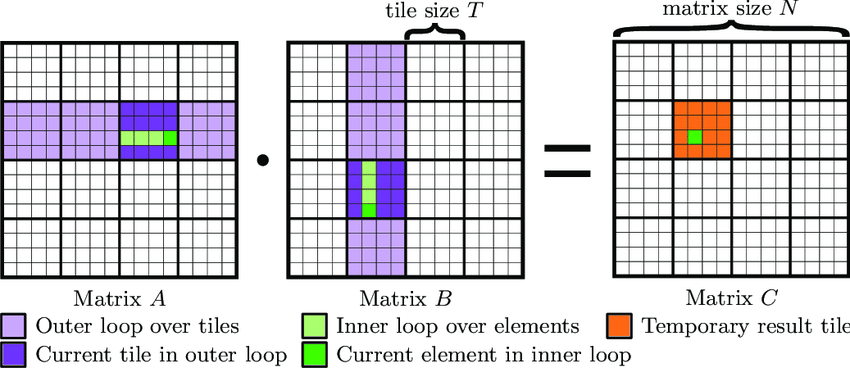 Tiling: each output tile of C is a thread block. Sweep the matching row-tiles of A and column-tiles of B, loading each into shared memory, accumulating into a partial sum, then write the tile to HBM. Source: CS336 Lecture 6.
Globally it looks like the naive approach (loop over tiles); locally each step looks like the idealized approach (multiply tiles already in shared memory). The kernel loops over K in steps of BLOCK_K, uses tl.dot on tiles, and — because we're already here — fuses the ReLU before writing out:
@triton.jit  # c = relu(a @ b); a is M×K, b is K×N
def matmul_relu_kernel(a_ptr, b_ptr, c_ptr, M, N, K, ...strides..., BLOCK_M, BLOCK_N, BLOCK_K):
    pid_m, pid_n = tl.program_id(0), tl.program_id(1)   # this output tile
    a_ptrs = a_ptr + idx_m[:,None]*stride_am + idx_k[None,:]*stride_ak
    b_ptrs = b_ptr + idx_k[:,None]*stride_bk + idx_n[None,:]*stride_bn
    acc = tl.zeros([BLOCK_M, BLOCK_N], dtype=tl.float32)
    for k in range(0, K, BLOCK_K):              # sweep row-tiles of A, col-tiles of B
        a = tl.load(a_ptrs, mask=...); b = tl.load(b_ptrs, mask=...)
        acc += tl.dot(a, b)                     # tiles in shared mem → looks like PyTorch
        a_ptrs += BLOCK_K * stride_ak; b_ptrs += BLOCK_K * stride_bk
    acc = tl.maximum(acc, 0.0)                 # fused ReLU
    tl.store(c_ptr + ..., acc, mask=...)
Strides make the index math work: a tensor is linearized in memory, and index = row·stride_row + col·stride_col (transposing just swaps the strides). Once tiles are in shared memory, tl.dot behaves like a normal matmul.
Golden rules & takeaways
Next: going beyond a single GPU — multi-GPU parallelism.
References
Primary source is the lecture (executable lecture_06.py). Tools & resources: