Where the memory and the FLOPs actually go

Opening note: the scaling-law forecast held

The Marin 1e23 FLOP run mentioned last lecture finished — and landed within ~0.05 loss of the pre-registered forecast. Each curve below is an IsoFLOPs sweep of smaller runs; you find the compute-optimal point, fit a scaling law, and predict the loss of a model you've never trained. Extrapolating the same recipe out to GPT-5-scale compute gives a concrete loss prediction (with the usual "your mileage may vary").

Marin 1e23 FLOP run matched its pre-registered scaling-law forecast. Source: CS336 Lecture 2 / W. Barr-Held.

First principles: why account at all?

The recurring goal — best model for a fixed compute/memory budget — means maximizing computational efficiency. But you can't optimize what you can't measure, so the prerequisite skill is understanding the compute and memory profile of a given computation. The point isn't to compute everything precisely; it's to get the rough shape of things from napkin math.

Caveat on the second: activations aren't counted (they depend on batch size and sequence length), so 53B is an upper bound. The 2 + 2 + (4 + 4) is parameters (bf16) + gradients (bf16) + Adam's two optimizer moments (fp32) — explained below.

Knowledge to take away: mechanics are straightforward (just PyTorch semantics), the mindset is to do resource accounting reflexively whenever you write a line of code, and the intuitions are just a feel for where resources go.

Tensors: the unit of everything

Every quantity in training — data, parameters, gradients, optimizer state, activations — is stored as a tensor. A tensor's rank is its number of dimensions: rank-1 is a vector, rank-2 a matrix, and Transformers routinely use rank-4 tensors (e.g. batch × sequence × heads × head-dim).

Memory is dead simple: (number of elements) × (bytes per element). A 4×8 fp32 matrix is 32 × 4 = 128 bytes. To feel the scale: a single feed-forward matrix in GPT-3 (49152 × 12288) is 2.3 GB — and that's an old, modest model.

Floating point: the precision/range/memory trade

Almost everything is a float, and the float type sets both memory and (often) speed. A float splits its bits into a sign, an exponent (dynamic range), and a mantissa/fraction (resolution).

fp32 — single precision (the default)

fp32 = 1 sign + 8 exponent + 23 mantissa bits = 4 bytes. The scientific-computing baseline; deep learning can be sloppier.

fp16 — half precision

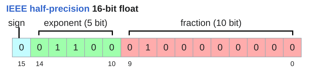fp16 = 1 + 5 + 10 = 2 bytes. Halves memory, but only 5 exponent bits → poor dynamic range.

The small exponent is dangerous: torch.tensor([1e-8], dtype=float16) rounds to 0 (underflow). Train in fp16 and you court underflow, overflow, and NaNs.

bf16 — brain floating point (Google, 2018)

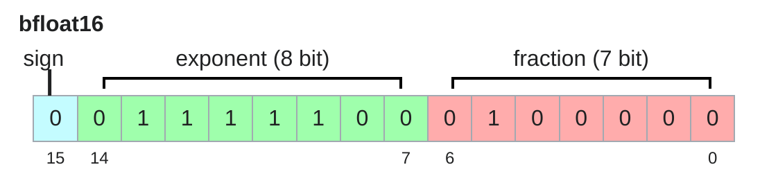bf16 = 1 + 8 + 7 = 2 bytes. Same memory as fp16 but borrows exponent bits back to match fp32's full dynamic range — at the cost of resolution.

bf16's insight: keep the bit count of fp16 but shift bits from mantissa to exponent. Result: same dynamic range as fp32, worse resolution — a trade deep learning happily takes (training is noisy/stochastic anyway). [1e-8] in bf16 does not underflow.

fp8 and fp4 — the frontier of low precision

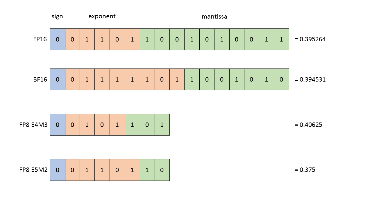fp8 (standardized 2022) comes in two flavors: E4M3 (more resolution, range [-448, 448]) and E5M2 (more range, [-57344, 57344]). Source: NVIDIA Transformer Engine.

In 2025 NVIDIA introduced nvfp4 — just 4 bits per value, with possible values {-6, -4, -3, -2, -1.5, -1, -0.5, 0, 0.5, 1, 1.5, 2, 3, 4, 6}. The trick: a separate scale factor per block, so an individual value gets more effective dynamic range than 4 bits would suggest — it just can't sit wildly far from its block-neighbors. The Nemotron 3 Super model (2026) was trained in nvfp4.

Mixed precision — best of both worlds

fp32 is safe but heavy; bf16/fp8 are light but risky. Mixed precision training uses each where it's safe:

• bf16 for parameters, activations, and gradients (the bulk of compute, e.g. matmuls).
• fp32 for optimizer states (accumulating squared/averaged values over many steps needs the resolution for stability).

PyTorch's AMP (torch.amp.autocast) wraps your code and auto-casts to bf16 when safe (matmuls) while keeping things like exp in fp32.

CPU vs GPU memory

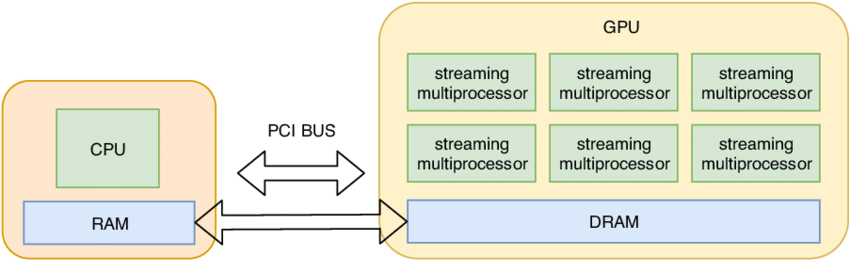Tensors live in CPU memory by default. To use the GPU's parallelism you must move them: x.to(device) — forget this and you lose your speed-ups.

An aside that pays off: einops

Index-based tensor code like x @ y.transpose(-2, -1) is easy to misread — what are dims -2, -1? einops names dimensions (inspired by Einstein summation), so you reason about meaning, not positions.

einsum — generalized matmul with bookkeeping

# Old way (what are -2, -1?):
z = x @ y.transpose(-2, -1)        # batch seq1 seq2

# einops way — name the axes; unnamed output dims are summed out:
z = einsum(x, y, "batch seq1 hidden, batch seq2 hidden -> batch seq1 seq2")

# '...' broadcasts over any number of leading dims (batch, heads, ...):
z = einsum(x, y, "... seq1 hidden, ... seq2 hidden -> ... seq1 seq2")

Note there's no transpose — the naming does the transpose for you. The ... lets you write modular code that works regardless of how many batch/head dims come in.

reduce — sum / mean / max / min

# Old: y = x.sum(dim=-1)
y = reduce(x, "... hidden -> ...", "sum")   # the dropped dim is reduced

rearrange — split / merge dimensions

# total_hidden actually packs (heads * hidden1); operate on one part:
x = rearrange(x, "... (heads hidden1) -> ... heads hidden1", heads=2)
x = einsum(x, w, "... hidden1, hidden1 hidden2 -> ... hidden2")
x = rearrange(x, "... heads hidden2 -> ... (heads hidden2)")

einops reduce is just sugar — it lowers to the same primitive ops, no speed difference. The payoff is that transposes and reductions stop being a source of bugs.

Counting FLOPs

A FLOP is one floating-point operation (an add or a multiply). Two maddeningly similar terms:

FLOPs (lowercase s)

Floating-point operations — a count of computation done. "Training GPT-3 took 3.14e23 FLOPs."

FLOP/s (per second)

Speed of hardware. "An H100 does ~1979 teraFLOP/s." Beware: spec sheets quote the number with sparsity — divide by 2 for dense (so H100 bf16 dense ≈ 9.9e14 FLOP/s).

For a linear layer mapping B points of dim D to K outputs (x [B×D] @ w [D×K]): one multiply and one add per (i,j,k) triple gives

FLOPs = 2 · B · D · K

Since D·K is the parameter count and B the number of points, this is the key identity: forward pass ≈ 2 · (#tokens) · (#parameters). Elementwise ops cost only O(mn), so for large enough matrices, nothing rivals matmul — which is why we mostly count matmuls (with a big asterisk for memory, next section).

Arithmetic intensity & the roofline

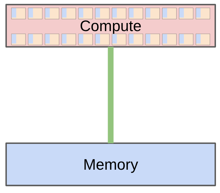The cartoon: tensors sit in high-bandwidth memory (HBM); to compute you (1) ship inputs to the accelerator, (2) compute, (3) ship outputs back. Memory is not where the compute is.

So runtime depends on two hardware numbers: accelerator speed (H100 ≈ 9.9e14 FLOP/s) and memory bandwidth (H100 ≈ 3.35 TB/s). We assume communication and computation perfectly overlap, so total time ≈ max(communication time, computation time).

Accelerator intensity

How much work the hardware can do per byte moved: FLOP/s ÷ bytes/s. For an H100 that's ≈ 295 FLOPs per byte — a number worth memorizing as "~300."

Arithmetic intensity (of an algorithm)

Work actually done per byte moved: FLOPs ÷ bytes.

The verdict falls out of comparing the two (equivalently, comparing communication vs computation time):

• Memory-bound: arithmetic intensity < accelerator intensity (you wait on bytes).
• Compute-bound: arithmetic intensity > accelerator intensity (you're saturating the cores).

Walking the common operations (all in bf16, so 2 bytes/value):

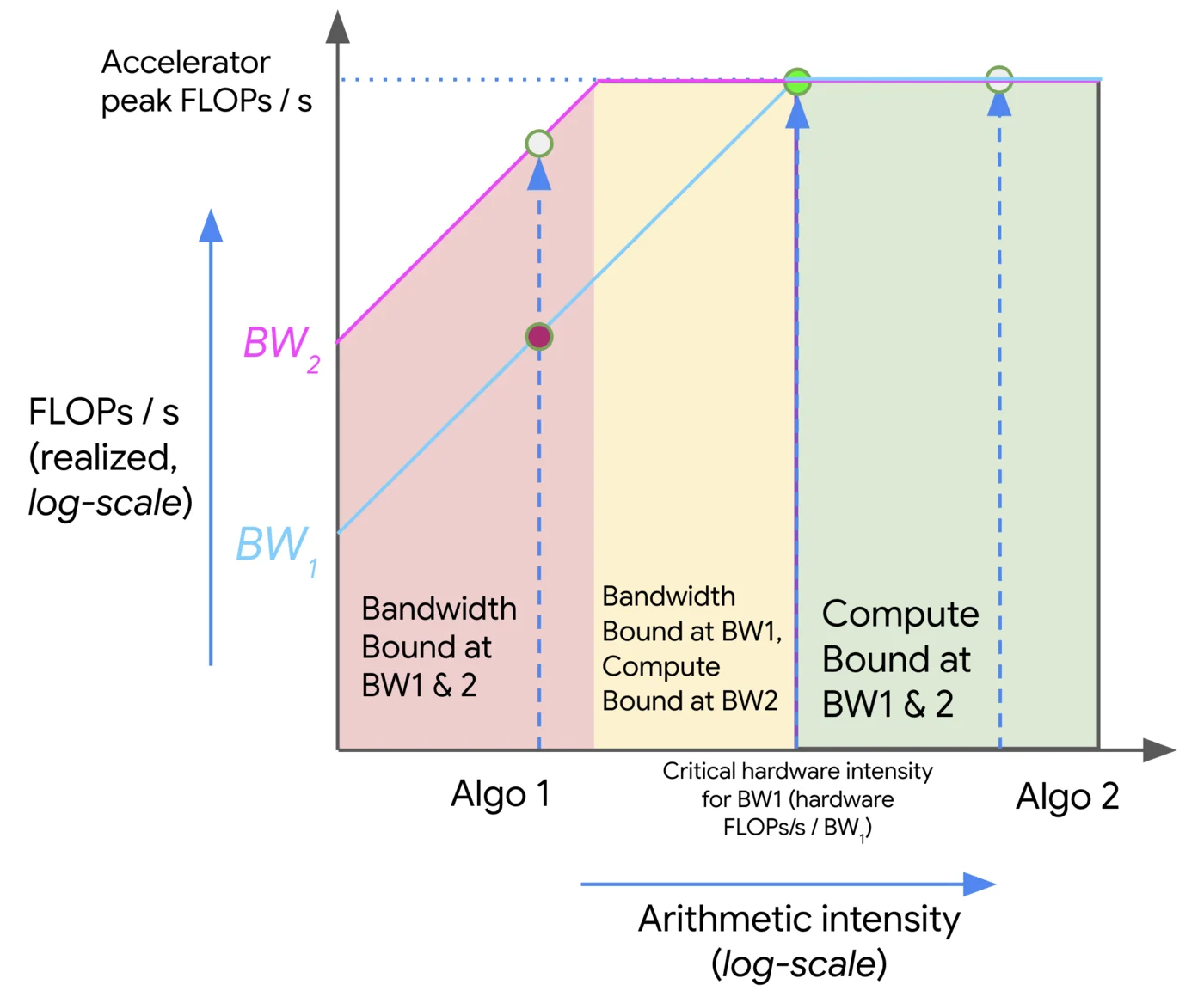Roofline plot: x-axis is arithmetic intensity, each sloped-then-flat line is a hardware device. Below the kink (the accelerator intensity) you're memory-bound and can't reach peak FLOP/s; above it you're compute-bound. Source: "How To Scale Your Model" (jax-ml).

This finally answers "why isn't MFU ~1?": MFU = min(1, arithmetic-intensity ÷ accelerator-intensity). Real workloads mix memory-bound ops in with the matmuls, dragging utilization down. Two corollaries: Transformers are mostly big matmuls (compute-bound — good news), but inference decodes one token at a time → matrix–vector products → memory-bound, which is why inference is hard. Intensity also depends on precision (bf16 vs fp32).

Gradients and the 6ND rule

A deep network: each layer is a D×D matmul + ReLU. The forward pass produces activations; the backward pass produces gradients for both inputs and parameters.

Backprop computes two things per layer. For a layer h2 = h1 @ w2, written in einsum so the shapes are unambiguous:

# backward message — gradient w.r.t. the input:
h1_grad = einsum(h2.grad, w2, "batch out, in out -> batch in")
# gradient w.r.t. the parameters:
w2_grad = einsum(h2.grad, h1, "batch out, batch in -> in out")

Each is a matmul over the same three dimensions, so each costs 2·B·D·D FLOPs — the backward pass is exactly 2× the forward pass (two gradients vs one product). einsum sidesteps the perennial "which one gets transposed?" confusion: you just match named dims.

That's where the famous 6ND comes from (N = params, D = tokens). It's derived here for MLPs but is a good approximation for Transformers too — until context length grows large, when the attention term adds an extra context² cost not captured by 6ND.

Optimizers and the memory budget

The optimizer family, built up by accretion:

SGD

Plain gradient step.

Momentum

SGD + exponential averaging of the gradient (first moment).

AdaGrad

SGD + averaging of the gradient squared (second moment); divide updates by √(Σ grad²). From 2011 — between SGD and Adam.

RMSProp

AdaGrad with exponential averaging of grad².

Adam

RMSProp + momentum (both first and second moments). You implement this in Assignment 1.

Now the full training-memory picture (bf16 params/grads, fp32 optimizer state):

Optimizer state must be fp32 because you accumulate averages over many steps — bf16 squares/averages are unstable. It eats a lot of memory, but note: optimizer state is not a compute bottleneck (it doesn't get shipped through matmuls). Its cost is purely "you can't fit a large model in HBM." Compute per step is just 6 · B · N. (Transformers: same idea, more bookkeeping — that's Assignment 1.)

Two ways to cut memory

Since activation memory scales with batch size — and you want large batches for stability up to a "critical batch size" (Tatsu, later) — you can run out of memory. Two standard fixes:

Gradient accumulation

Split a batch into micro-batches, compute gradients on each, and accumulate them (don't zero out). Every batch_size ÷ micro_batch_size steps, update the parameters and zero the gradients. A tiny code change that decouples the effective batch size from activation memory.

Activation checkpointing (a.k.a. gradient checkpointing / rematerialization)

By default training stores every layer's activations for the backward pass (inference doesn't, since no gradients). The idea: in the forward pass keep activations only at a subset of layers; in the backward pass recompute the missing ones from the last checkpoint. Classic trade of compute for memory (torch.utils.checkpoint.checkpoint(layer, x)).

Checkpointing every √L layers is the balanced sweet spot.

Golden rules & takeaways

• Everything is tensor operations — parameters, gradients, activations, optimizer states, data — and memory is just (#elements × bytes/element).
• 6 · (#data points) · (#parameters) FLOPs per training step (forward 2, backward 4). Holds for Transformers at modest context length.
• Diagnose with arithmetic intensity / roofline. Matrix multiplications are compute-bound; essentially everything elementwise is memory-bound — so the cost of an op is often "how many bytes did it move," not "how much math did it do."
• bf16 is the sweet spot (fp32 range, half the memory); keep optimizer states in fp32; let AMP handle the casting.
• Gradient accumulation and activation checkpointing trade compute for memory, letting you use bigger batch sizes than would otherwise fit.
• Adopt einops. Naming dimensions removes a whole class of transpose/reduction bugs.

Next lecture: Tatsu on Transformer architectures.

References

Primary source is the lecture itself (and its open-source trace); diagrams are reproduced from the course materials. External works named in the lecture:

1. CS336 Lecture 2 source (resource accounting) — executable lecture
2. Micikevicius et al. (2017) — Mixed Precision Training
3. Micikevicius et al. (2022) — FP8 Formats for Deep Learning
4. NVIDIA — Introducing NVFP4 (4-bit)
5. Duchi, Hazan & Singer (2011) — Adaptive Subgradient Methods (AdaGrad)
6. Austin et al. — How To Scale Your Model: roofline analysis
7. Transformer training memory (blog) · Transformer FLOPs (blog)