Why build from scratch — and the atoms a model sees
Two things in one lecture: why this course teaches you to build language models from the ground up (and what of that actually survives the jump to frontier scale), and the first concrete building block — the tokenizer, which decides what "atoms" the model ever gets to reason about.
First principles: why a "from scratch" course exists
The whole premise is that you understand language models by building every layer yourself. You won't literally build everything — that wouldn't fit in a quarter — so the course is a refined recipe of the highest-value pieces to construct by hand.1
The motivation is a worry about abstraction drift. The field has steadily moved up the abstraction ladder: ~10 years ago every AI researcher implemented and trained their own models; ~8 years ago people downloaded a pre-trained model (BERT) and fine-tuned it; today you can get a long way just by prompting. Moving up abstractions is genuinely good — but abstractions are leaky. You eventually hit a wall where the model can't do what you need and prompting gives you no recourse. For fundamental research, prompting also silently shrinks your design space: to do real fundamental work you have to be able to tear up the whole stack.
Full understanding of how language models work is necessary for fundamental research, and the way you reach that understanding is by building. That single sentence is the philosophy of the entire class.
The industrialization problem
There's a catch: language models have industrialized. Frontier models are enormously expensive and completely closed. GPT-4 reportedly cost on the order of $100M three years ago; current frontier runs are plausibly on the order of $1B. The GPT-4 report explicitly declined to share any architectural or training detail, citing the competitive landscape and safety. So the frontier itself is out of reach for a course.
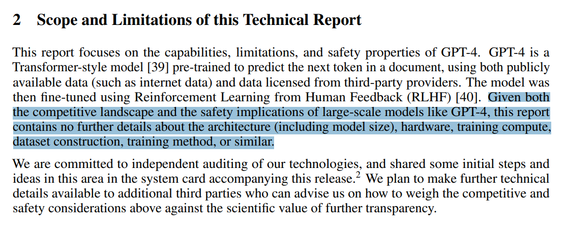 The GPT-4 technical report, stating plainly that no details of architecture, data, or training will be disclosed — citing competition and safety.
The instructor flagged the ~$100M and ~$1B numbers as unconfirmed/estimated, not disclosed figures. Treat them as order-of-magnitude intuition, not precise facts — and note they will keep drifting upward over time.
We can — and will — build small language models. But small models are not guaranteed to be representative of frontier models, and two concrete phenomena show why:
- 1 · Where the FLOPs go changes with scale
- At small scale the MLP layers consume ~44% of FLOPs; scale up to 175B parameters and that rises to ~80%. So what is worth optimizing differs by scale — tune attention hard at small scale and the win may simply not appear at large scale.
- 2 · Emergence
- On zero-/few-shot tasks, small models look like nothing is working at all; only past a critical scale does performance suddenly jump. Whole classes of behavior are invisible at small scale.
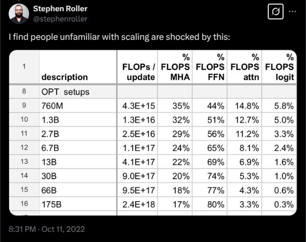 Example 1: the share of FLOPs in attention vs MLP shifts with scale (S. Roller).
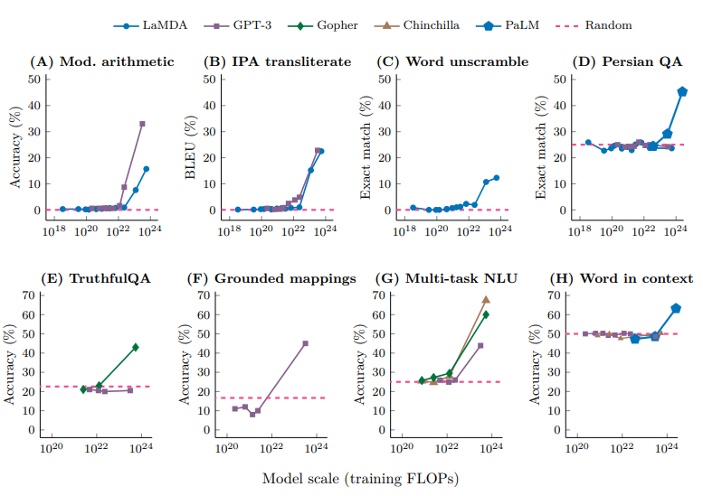 Example 2: emergence — capabilities stay flat, then jump past a critical scale (Wei et al.).
The 44%→80% FLOP split and the emergence curves are drawn from older results (≈2020–2021). They make the conceptual point; the exact percentages should not be read as current architecture-specific facts.
So what actually transfers?
If we can't touch the frontier, the honest question is which knowledge survives the jump in scale. Break it into three kinds:
| Knowledge | What it is | Transfers to scale? |
|---|---|---|
| mechanics | How things work — what a transformer is, how model parallelism works | Yes — provable by construction |
| mindset | How to approach building — profile everything, benchmark, take efficiency and scaling seriously | Yes |
| intuitions | Which modeling / data decisions actually yield good performance | Not reliably — needs scale to learn |
The course can teach mechanics and mindset well, and it will relentlessly emphasize profiling, benchmarking, and optimizing for efficiency. Intuitions about what works often can't be justified analytically — they come only from running experiments. The canonical confession is Noam Shazeer's SwiGLU paper, whose conclusion offers no explanation for why the architecture works and attributes its success "to divine benevolence."6 Mechanics you can see; intuitions you have to earn.
 The actual conclusion of Shazeer's GLU-variants paper — an unusually honest admission that some architecture wins are purely empirical.
The mental model: the bitter lesson, read correctly
The "bitter lesson"7 is widely misquoted. The wrong reading is "scale is all that matters, algorithms don't." The right reading is: algorithms that scale are what matter. A simple decomposition makes this precise:
output / input
input
Efficiency matters more as scale grows. At small scale, a run that takes twice as long just means you wait and come back later. At large scale that can be hundreds of millions of dollars — so even a 5% efficiency gain is a big deal. Empirically the algorithmic side is huge: OpenAI measured ~44× algorithmic-efficiency improvement on ImageNet between 2012 and 2019, on top of hardware gains. Multiply the two and you get the dramatic jumps in accuracy.
What is the best model you can build with a given data and compute budget? For pre-training we'll mostly reason about the compute budget (assuming data is more plentiful than compute) — but if you're data-limited, or you've stashed away a pile of B200s, you may instead be data-bound. Either way: maximize efficiency.
A short history, so the present makes sense
Language models are old. Shannon used them in the 1950s to measure the entropy of English, and for decades n-gram models were a core component of machine translation and speech recognition — not the whole system, but the part that kept generated text fluent.
The lineage of modern models is neural:
1990s
first neural LM
+ MoE, parallelism
Yoshua Bengio wrote the first neural language model in 2003 — a feed-forward network over a small context, not an LSTM.9 Then Seq2Seq boldly compressed a whole sentence into a vector; the Adam optimizer and the attention mechanism arrived (attention built for machine translation), the transformer built on attention (also for MT), and the 2010s piled on architecture, systems, and optimizer ideas.
By the late 2010s things got interesting. ELMo and BERT were trained on lots of text, then fine-tuned on downstream tasks like question answering for big gains — the model was something you fine-tuned. A Google paper foreshadowed the "prompt in, response out" view. Then OpenAI opened the floodgates by embracing scaling: GPT (2018) → GPT-2 → and crucially the discovery of scaling laws,4 which enabled GPT-3 — more than 10× the largest model at the time — and surfaced emergent in-context learning.10 Google's response was a massive model that turned out undertrained, while DeepMind (then separate) worked out compute-optimal scaling.5
GPT-3 was a wake-up call. Early replication attempts — Eleuther's grassroots open datasets/models (small, compute-starved), Meta's first 175B LLM (a visible replication, but weak and plagued by hardware issues), and Hugging Face's BigScience — were not very strong. Over the last three years the open ecosystem changed dramatically: Meta's Llama / Llama 2 / Llama 3, Mistral, and a wave of Chinese models (DeepSeek, Qwen, and others from ByteDance, Tencent, …). Open-weight models now approach closed ones and are widely used in industry. A further step goes beyond open weights to fully open — AI2, NVIDIA, and the Marin project release weights plus paper, code, and data.
This course is only possible because of open models and the papers around big MoE and RL systems — they let us glimpse and triangulate how frontier models are built. The details are still incomplete (e.g., Qwen papers omit the data mixture, so you can't truly reproduce them) — but far better than nothing.
The idea of what a language model "is" kept shifting — something you fine-tune → something you prompt → (ChatGPT era) something you talk to → (now) an agent that runs long, complex coding tasks from a page of instructions. Yet the fundamentals barely moved: still GPUs and kernels, still gradient/SGD-style optimization, still the transformer and attention. What changed are the specs — far longer context lengths, which makes inference efficiency matter more than ever.
The five parts (and five assignments)
The course mirrors the pipeline of actually building a model. Each part is one assignment.
Part 1 · Basics — train a model from scratch
First two weeks. Goal: tokenize the data, define the architecture, implement the optimizer, and train. Three sub-problems:
Tokenization
Decides the atoms the model operates on (the full second half of this lecture). Through the efficiency lens it both shortens the sequence and — more importantly — enables adaptive computation: common stretches collapse to one token, rare/interesting stretches stay multi-token.
Architecture
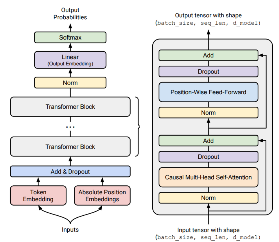 The starting point: the original Transformer (Vaswani et al., 2017). Everything that follows is a refinement of this.
The transformer, familiar from CS224N, but with many refinements since: activation functions evolved, positional encodings evolved, normalization (where and how) evolved. Full attention is O(n²) in sequence length and gets expensive, so there are many attention-reduction schemes; more ambitiously, state-space / linear-attention models (Mamba, Gated DeltaNet) have grown popular, and a hybrid of these with attention often works best. Inside the MLP, the original dense layer has largely given way to mixture-of-experts (MoE) as the dominant compute-efficient design — which also demands different training techniques. Finally the "shape" — number of layers, heads, hidden dimension, number of experts — looks like trivial hyperparameters but has outsized impact once scaling is involved.
Training
Design decisions around the loss and optimizer:
These look like "just hyperparameters," but setting them principledly is the difference between a run that blows up and one that reaches state of the art.
Tokenizer, model, and training look like separate pieces, but they're all one balancing act between three forces: expressivity (represent the data's complexity), stability (keep parameter and gradient norms in a goldilocks zone — not exploding, not vanishing; much of training LMs is really about stability), and efficiency (run fast on hardware). Most architecture choices are "make it faster by projecting to a lower-dimensional space — but does it still work as well?" Making those trade-offs is the game.
Assignment 1: implement the BPE tokenizer, the transformer, the loss, the optimizer, and the full training step; do resource accounting; train on TinyStories and OpenWebText; then a leaderboard to drive perplexity down as fast as possible (in the spirit of NanoGPT speedruns).
Part 2 · Systems — get the most out of the hardware
Kernels, multi-GPU parallelism, and inference.
Resource accounting (starts next lecture)
Track exactly where every FLOP and every byte of memory goes. The headline formula: training an N-parameter model on D tokens costs roughly 6 · N · D FLOPs — and we'll derive where that comes from. The hardware cartoon to hold in your head: memory is not where the compute is. You must move parameters/activations from memory to the compute units and back, and that movement is often the bottleneck. Example: a B200 offers ~2.25 PFLOP/s (bf16) but ~8 TB/s of memory bandwidth — the mismatch is the whole story. Roofline analysis tells you whether a computation is compute-bound or memory-bound (usually memory).
The B200 throughput/bandwidth figures are current-generation reference points used for the math. The method (roofline, 6ND) is durable; the specific numbers will be superseded by newer accelerators.
Kernels
A kernel is a function that runs on the GPU. Plain PyTorch primitives already launch built-in kernels — you're using kernels whether you realize it or not. For certain computations, custom kernels go faster, and the governing principle is minimize data movement. Compute A·B naively and you read from HBM, compute, write back, read again, compute, write back — moving data twice. Operator fusion reads once, does both computations, writes once. Tiling is a more sophisticated variant of the same idea. We'll write kernels in Triton.
Many GPUs
Same principle, but moving data between GPUs is even more expensive. The classic collective operations — gather, reduce, all-reduce — are the vocabulary of distributed training. The game: shard model parameters, activations, gradients, and optimizer states across GPUs, then orchestrate bringing the right data to the right node, computing, and writing back. You can shard by data, model, layers, sequences, or experts, each with trade-offs. (A DGX B200 is 8 GPUs on NVLink; a thousand-GPU cluster wires many such boxes together with InfiniBand or Ethernet.)
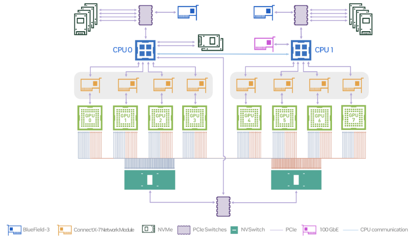 A DGX B200 node: 8 GPUs fully connected by NVLink, with NICs for InfiniBand/Ethernet across nodes. Source: NVIDIA DGX B200 user guide.
Inference
Using the model — for chatting, but also RL rollouts, test-time compute, synthetic-data generation, and evaluation, so it's increasingly central. Two phases:
feed the whole prompt, build KV cache — like training
one token at a time — quickly memory-bound
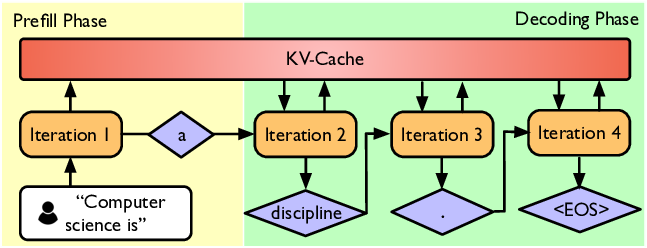 Inference's two phases: prefill processes the whole prompt at once (compute-bound, like training); decode emits one token at a time (memory-bound).
Decode is where inference gets hard. Speedups: use a cheaper model (prune, quantize, distill); speculative decoding (a cheap model races ahead guessing tokens, the full model verifies them in parallel and accepts the lucky ones — beating one-at-a-time); inference-specific kernels; and batching queries that arrive at unpredictable times (unlike training, where batches are predefined).
Assignment 2: implement kernels in Triton and do parallel training (details may shift as the staff revamp the systems assignment). Highly recommended companion: the Google "How to Scale Your Model" book — great for roofline analysis and transformer math; it's TPU-focused but the concepts carry, and it now has a GPU chapter.8
Part 3 · Scaling laws — predict before you spend
Imagine you have 1e25 FLOPs (tens of millions of dollars). What model do you train? You can't hyperparameter-tune at that scale because you only get to train one model — and mistakes are money down the drain. This is the problem you simply never face when fine-tuning or doing small-scale work.
Stop thinking about a single model; think about a scaling recipe — a mapping from a FLOP budget to a set of hyperparameters (essentially a config file). For a given recipe, run small-scale experiments, measure loss, fit a scaling law, and use it to predict the loss at the target scale. Then you can (a) optimize the recipe for large scale using only cheap experiments, and (b) predict the loss before committing — which is, not incidentally, how you raise the money to do the run.
A crucial corrective: scaling laws are not laws of nature. They don't happen automatically — you will them into existence by carefully constructing a recipe that extrapolates (e.g., how the learning rate holds or drops and how batch size grows as scale increases). To make predictions hold, you parameterize the model for hyperparameter transfer: the hyperparameters at small scale are either the same at large scale or a predictable function of it. Otherwise you can't possibly guess the right learning rate at the top.
So a mindset shift: predictability is at least as important as optimality. You still want optimal/efficient settings, but you also want to never be surprised at scale.
The actual laws are fairly classic. Given a FLOP budget, how do you balance a bigger model against more tokens? This is the Kaplan compute-optimal4 / Chinchilla5 question. For each FLOP budget (say 6e18 up to 3e21) you sweep model sizes, pick the best, then fit a curve predicting #params from budget. If the points lie on a line, great; if they're scattered, you have no business trusting your extrapolation. The crude rule of thumb: ~20 tokens per parameter — so a 70B model wants ~1.4T tokens.
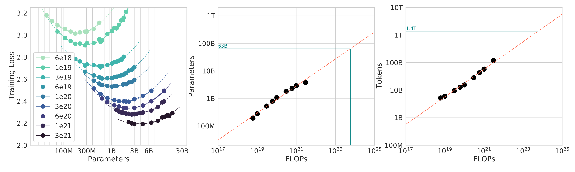 Classic compute-optimal scaling: for each FLOP budget, an IsoFLOP curve locates the optimal model size; fitting across budgets extrapolates to large scale (Chinchilla).
It varies with dataset and architecture, and it ignores inference cost. Many modern models are deliberately small but trained on far more tokens than compute-optimal, precisely to be cheap at inference.
Assignment 3: a training "API" — submit a config, get a loss back. The staff trained many models offline and cache the results so it feels like training. You fit scaling laws to the points, extrapolate, and then they evaluate how well your chosen large-scale config actually lands — a low-stakes simulation of a high-stakes $100M decision.
Part 4 · Data — what you train on is what you get
Arguably the most important part: data quality basically specifies how good the model will be, and data reflects what you want the model to do (speak many languages? converse? run long agentic coding tasks?).
Evaluation first
Evaluation defines the capabilities you're aiming for, and it's deeper than "run some benchmarks." Two distinct purposes that often get conflated:
| Type | Purpose | What matters |
|---|---|---|
| Internal metrics | Model development | Smoothness across scales (predictability) and relative performance — absolute numbers like "perplexity 1.2" mean little on their own |
| External metrics | Reporting to customers / reviewers | Ecological validity |
Perplexity remains an excellent internal signal of intrinsic model quality without benchmark fuss. A separate question is what you evaluate on: data not on the internet is ideal, to avoid contamination. Because language models are purportedly general-purpose, you want a diverse set of evals — you can average them into one number, but the average conflates many different things.
Getting and processing data
Data doesn't fall from the sky; it must be actively curated. Sources include crawled web pages, books (legally contentious), arXiv, and GitHub code.
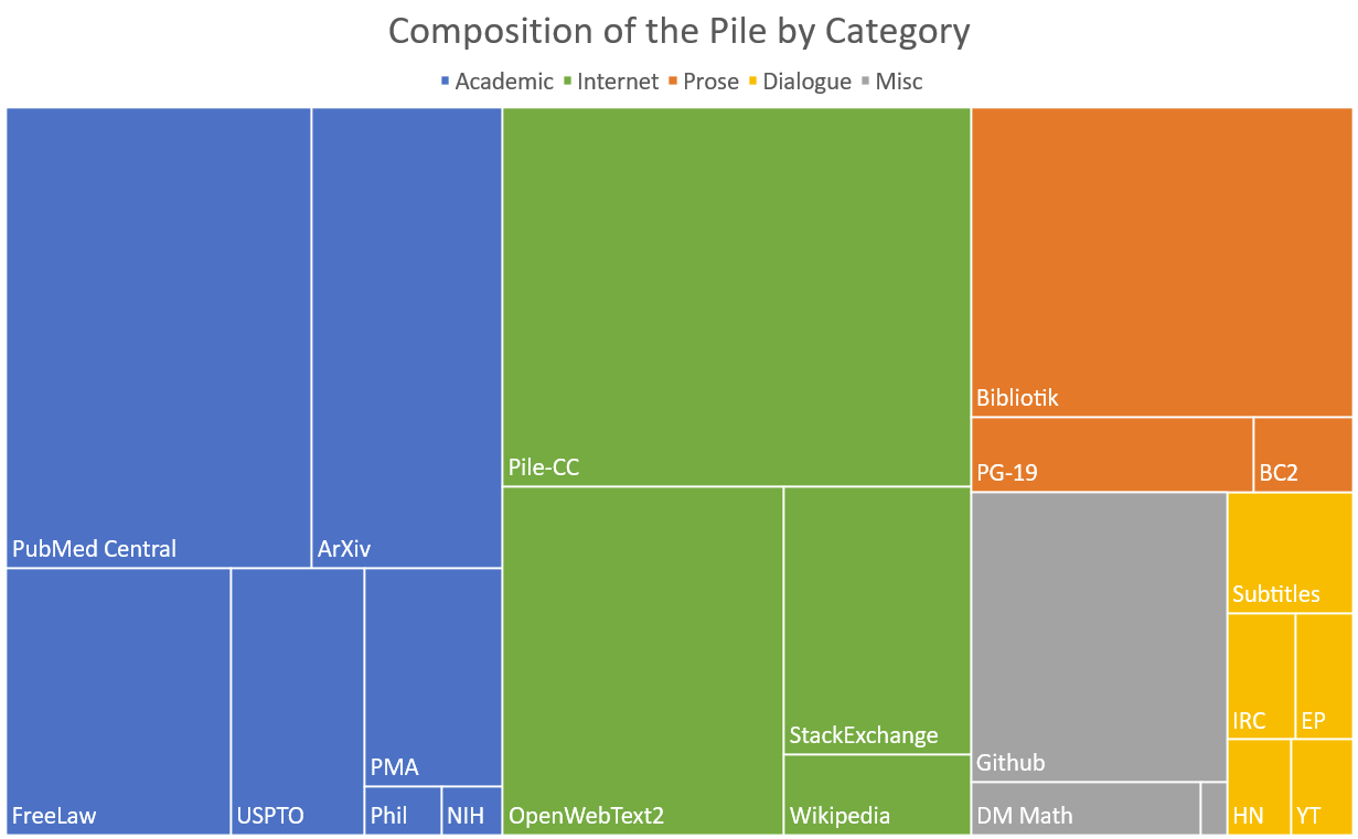 Language-modeling corpora are diverse: the composition of The Pile (2021) by source — web, books, code, academic, and more.
There are real legal issues — is training on copyrighted data fair use? what about GitHub code with no license: assume permissive, or be conservative? And raw data isn't even text — it's HTML, PDFs, code directories — so it needs processing:
non-text → text
keep the good stuff
combine sources
rewrite real data
Synthetic data — rewriting real data into something more Wikipedia-like or more like the downstream task — is an active research area. And data feeds several stages: pre-training, mid-training (high-quality data placed at the end of pre-training, including long-context data like big code repos and books), and post-training (conversations, agentic traces with tool calls).
Assignment 4: start from a raw web crawl and do all the filtering and deduplication to make it clean. "Dirty work," but it's a real part of building a model from scratch.
Part 5 · Alignment — improve with weak supervision
So far everything used full supervision (predict the next token[s]). The model is already reasonable, but you can push further with weak supervision, motivated by a simple asymmetry: it's often easier to critique than to generate. You can't always provide the one right response to a prompt, but you can often specify what "good" looks like. The template:
responses from the model
human · verifier · LM judge
prefer better responses
Instantiated via RL algorithms (PPO GRPO) or, for preference data, DPO. The challenges: RL is unstable and hard to tune — the instructors' preference is to stay in the fully-supervised regime as long as possible. And RL at scale adds serious systems problems: you run an inference server (generating rollouts, sometimes against environments that execute code) alongside a training server; when workers lag you drift off-policy, so you're perpetually juggling on-policyness against throughput. "A big, wonderful mess."
Assignment 5: still being finalized; last year it was implementing DPO and GRPO and getting them working on a math benchmark, with plans to push further toward realistic settings this year.
The thread tying it all together: efficiency
Every design decision in the course can be read as optimizing efficiency — either data efficiency or compute efficiency — given fixed resources (data, compute cores, memory, communication bandwidth).
- Systems
- Directly about compute efficiency.
- Tokenization
- Raw bytes are compute-inefficient for today's architectures; tokenization buys efficiency.
- Architecture
- Most changes reduce memory or FLOPs — many specifically to speed up inference.
- Data filtering
- Don't spend gradient steps on redundant bad data; under a fixed compute budget, time on bad data is time stolen from good data.
- Scaling laws
- Effective hyperparameter tuning done on much smaller (cheaper) models.
Tomorrow the world may become data-constrained and the calculus of which decisions to make will change — but the durable mindset the course wants to install is: always think about the efficiency of your approach.
Course logistics (for completeness)
5 units, 5 intense assignments (the first alone is said to rival all of CS224N's). Take it if you have an obsessive need to understand how things work — you'll come out with strong research/engineering muscles and the confidence to handle any new setting. Don't take it if you need to ship research this quarter (tell your advisor), if you want the hottest new techniques (no multimodality, no deep dive on agents — other seminars fit better), or if you have an application to ship (prompt → fine-tune → and only as a last resort pre-train). Assignments give no scaffolding code but plenty of unit tests, are largely doable on a laptop with a provided cluster (Modal credits this year) for real training/benchmarking runs, and most have leaderboards. AI policy: coding agents could solve the assignments outright, so they provide a pedagogically-minded AGENTS.md prompt — use AI with it, so it tutors and answers questions without handing you the transformer you're supposed to write.
What are the atoms the model operates on?
The first real building block. Andrej Karpathy's "Let's build the GPT Tokenizer" is the recommended companion video.2
The job of a tokenizer
Raw text is a Unicode string. A language model places a distribution over sequences of tokens, usually represented as integer indices. So we need a procedure to encode strings into tokens and decode tokens back into strings. A tokenizer is whatever can do that round trip.
"the cat"
[256, 99, 97, 116]
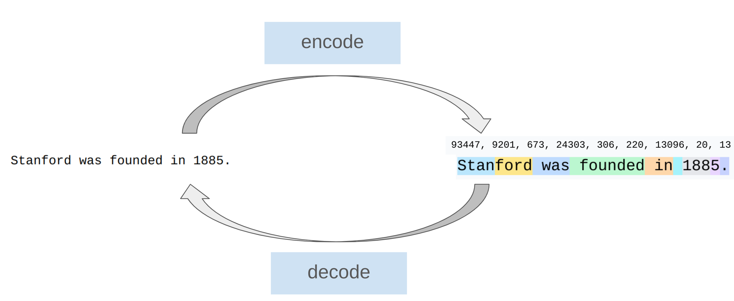 A real tokenization: text broken into tokens (each colored span is one token, one integer index).
Encode then decode must return the original string. If your tokenizer doesn't round-trip, you have a bug.
Playing with real tokenizers reveals why people find them annoying. A word and the same word with a preceding space are different tokens — many tokens are literally "space + word" — so "hello" and " hello" are completely different indices with nothing to do with each other. Numbers are erratic: some tokenizers chunk every few digits (sometimes predictably, sometimes not), others make every digit its own token, which blows up the token count. There's a trade-off everywhere.
The metric: compression ratio
Define compression ratio = bytes / tokens. For a 20-byte string encoded into 8 tokens, the ratio is 20 / 8 = 2.5 bytes per token. A larger ratio means a shorter sequence, which is good because attention is quadratic in sequence length — shorter sequences are cheaper.
You can raise the compression ratio by growing the vocabulary — but then you hit sparsity, because every vocab element is treated as a distinct, independent symbol. Modern (especially multilingual) tokenizers land around 100k–200k tokens as a compromise.
Four ways to build one — three bad, one good
The lecture builds up by elimination. Each approach fails on the vocab-size ↔ compression trade-off in its own way.
1 · Character-level
A Unicode string is a sequence of characters; each character is an integer (Python's ord), reversible back to the character. Encode each character as a token. It round-trips fine — but there are ~150k Unicode characters, so the vocabulary could be ~150k (large, though not insane). The real problem: many characters are rare, so the vocabulary is used inefficiently, and the compression ratio is poor — you spend many tokens per string while most indices barely appear.
2 · Byte-level
Encode the string to bytes via UTF-8: "a" is 1 byte, other characters take several. Now every value is in 0–255, so the vocabulary is tiny — but the sequence is long and the compression ratio is 1, which is bad. Small vocab, very long sequences.
3 · Word-level
What classical NLP did: split on spaces or a regex and call each chunk a token. Each token is meaningful (humans invented words; words carry stable semantics) and compression is good. But the vocabulary is the number of distinct chunks in the training data — potentially huge, and in fact unbounded: at test time you'll meet a chunk you've never seen. The old fix was an UNK token, which is ugly and corrupts perplexity calculations.
4 · Byte-Pair Encoding (BPE) — what we actually use
BPE was invented long ago for data compression, brought into NLP for neural machine translation,3 and first used for LLMs in GPT-2 (Radford et al., 2019). You train the tokenizer on raw text to build a vocabulary tailored to the data, with a lovely property: everything is tokenizable — common sequences become a single token, and rare sequences split into smaller units, so there's no UNK.
The BPE training algorithm
Conceptually simple: start from the byte sequence (each byte is a token), then repeatedly merge the most frequent adjacent pair into a new token.
# Train: repeatedly merge the most frequent adjacent pair.
indices = list(text.encode("utf-8"))   # bytes -> ints in 0..255
merges  = {}                            # (a, b) -> new_id
vocab   = {i: bytes([i]) for i in range(256)}

for new_id in range(256, vocab_size):
    counts = count_pairs(indices)      # how often each adjacent pair occurs
    pair   = max(counts, key=counts.get) # most frequent pair (ties -> first)
    indices = merge(indices, pair, new_id) # replace every occurrence of pair
    merges[pair]    = new_id
    vocab[new_id]   = vocab[pair[0]] + vocab[pair[1]]
Walking through "the cat in the hat":
- Convert to a byte sequence. Count adjacent pairs; the pair (116, 104) — i.e. t,h — occurs twice (the most, ties broken by taking the first).
- Merge it: create new token 256 standing for "th", add it to the vocabulary, and replace every (116, 104) in the sequence with 256.
- Iterate. Next the most frequent pair is (256, 101) = "th" + "e" → new token 257 = "the". One more merge produces 258, and so on.
Each iteration the sequence shrinks and the vocabulary grows. On this toy string the compression ratio reaches about 1.5. Common byte sequences condense to single tokens; rare ones stay split.
Encoding new text (and decoding back)
To tokenize a new string, apply the learned merges to it, in the order they were learned; decoding reverses the process and returns the original string.
# Encode: apply learned merges in order.
indices = list(text.encode("utf-8"))
for pair, new_id in merges.items():     # SLOW: loops over EVERY merge
    indices = merge(indices, pair, new_id)
return indices # e.g. encoding of "the quick brown fox"It loops over all merges (and the number of merges is essentially vocab_size − 256). Assignment 1 asks you to make it fast: only loop over the merges that actually matter, building indices to find them. There are also special tokens to handle (not conceptually deep, but required for a modern tokenizer), and in practice you first break the text into chunks and tokenize each chunk — much faster than tokenizing one giant string. If Python proves too slow, reimplement the hot path in Rust or C.
Comparison: the four tokenizers
| Approach | Vocab size | Compression | Fatal flaw — vs the alternatives |
|---|---|---|---|
| Character | ~150k | poor | Rare chars waste the vocab · vs byte (smaller vocab) · vs BPE (data-driven sizing) |
| Byte (UTF-8) | 256 | 1.0 | Sequences far too long · vs word (meaningful units) · vs BPE (merges shorten) |
| Word | unbounded | good | Unbounded vocab + UNK at test time · vs char/byte (closed vocab) · vs BPE (no UNK) |
| BPE | ~100–200k | good | Needs training + a tokenizer stage at all · vs char/byte/word (all worse on the trade-off) |
Golden rules & takeaways
Even an end-to-end replacement has to satisfy two properties. (1) The transformer must operate on some abstraction of the sequence — most obvious for video or DNA, where individual bytes are low signal-to-noise and you must lift them into a space where modeling makes sense. (2) Chunks must be variable-length, enabling adaptive computation — not all bytes deserve equal treatment. Miss either and you'll be suboptimal.
Next lecture: resource accounting ("baby systems") — where the FLOPs and memory actually go — then on to architectures.
References
Primary source is the lecture itself; the items below are the external works it names.
- CS336: Language Modeling from Scratch — course website (Stanford)
- Andrej Karpathy — "Let's build the GPT Tokenizer"
- Sennrich, Haddow & Birch (2016) — Neural Machine Translation of Rare Words with Subword Units (BPE)
- Kaplan et al. (2020) — Scaling Laws for Neural Language Models
- Hoffmann et al. (2022) — Training Compute-Optimal Large Language Models (Chinchilla)
- Shazeer (2020) — GLU Variants Improve Transformer ("divine benevolence")
- Sutton (2019) — The Bitter Lesson
- Austin et al. — How To Scale Your Model (Google DeepMind)
- Bengio et al. (2003) — A Neural Probabilistic Language Model
- Brown et al. (2020) — Language Models are Few-Shot Learners (GPT-3)