CS336 · Lecture 14 — Data II (Pipeline & Post-training)

Transformation: raw data isn't text

Common Crawl is HTML; arXiv is PDF; GitHub is directories. The big one is HTML → text: remove boilerplate (nav, ads), extract the main content, and decide what to do with images/tables. It's inherently lossy — you linearize a hierarchical/visual document into a token sequence (nested tables are especially painful). Done with fast rule-based tools (trafilatura, resiliparse, jusText), and the tool choice measurably affects downstream accuracy.

PDFs (FinePDFs) are a small but high-value slice — if someone made a PDF, they probably had something to say. They need recrawling (PDFs are big and often truncated in Common Crawl) and OCR via a VLM (expensive), and they lose the semantic layout tags HTML provides.

The one framework

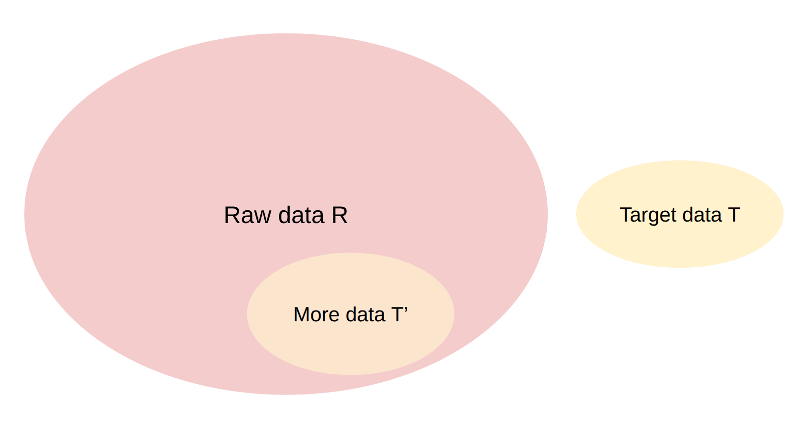Given a small amount of target data T and a huge pile of raw data R, find the subset of R that looks like T. Source: CS336 Lecture 14.

Almost all filtering fits this skeleton, with two requirements: generalize from T (don't just recover T) and be extremely fast (you run it on ~100T tokens). The recipe: estimate a model from R and T, derive a score, keep examples above a threshold (often stochastically). Two classifier types:

# Generative model of the target (e.g., KenLM 5-gram): score(x) = p_T(x)
# Discriminative classifier (e.g., fastText, a linear bag-of-words): score(x) = p(T | x)
#   positives = T;  negatives = random sample of R;  keep x if score(x) ≥ threshold

Early datasets avoided model-based filtering to dodge bias (C4, Gopher, RefinedWeb, FineWeb, Dolma); now it's the norm (GPT-3, LLaMA, DCLM) — unless you're compute-rich, you can't afford to waste FLOPs on junk.

Application / dataset	Target (positives)
Language ID (fastText, 176 langs)	multilingual sites; Dolma keeps p(English) ≥ 0.5
OpenMathText	rules (LaTeX) + KenLM on ProofPile + fastText math classifier → 14.7B tokens beat 20× unfiltered data
GPT-3	Wikipedia/WebText/Books vs Common Crawl (Pareto-stochastic keep)
LLaMA	pages referenced by Wikipedia vs Common Crawl
phi-1	GPT-4 scores "educational value" on 100K → random-forest classifier → HumanEval 12% → 18%
Toxicity (Dolma)	Jigsaw toxic-comments dataset

⚠️ There's no single optimal filtering threshold

It depends on how long you'll train. Train longer → tolerate lower-quality data; train shorter → demand higher quality. Empirically: heavily-filtered data wins early but, once you start epoching it, low-quality data trained longer eventually wins (more tokens beats repeating high-quality data). So filtering aggressiveness is a function of your token budget.

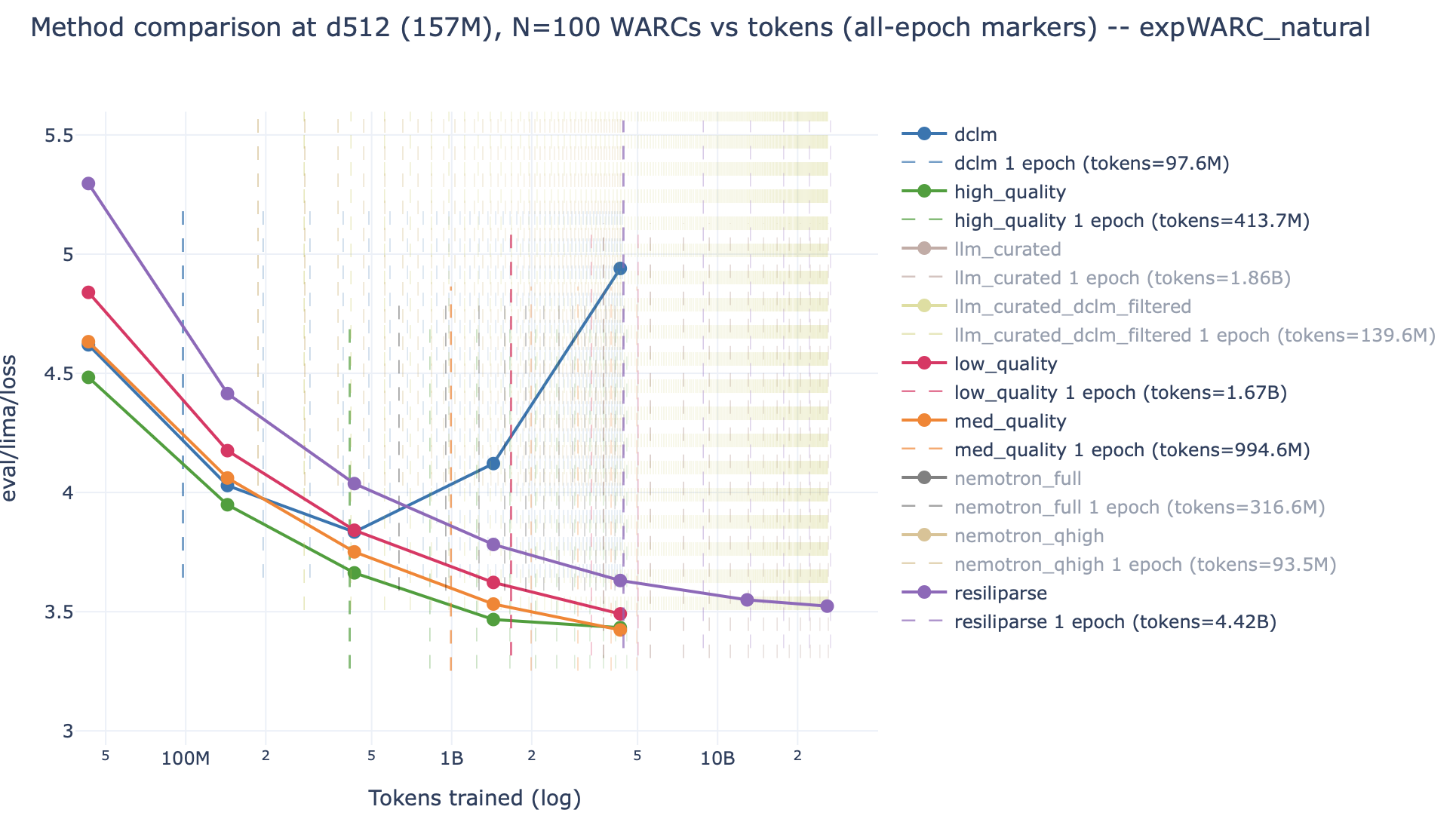High-quality vs low-quality data loss curves with epoching

High-quality (DCLM) starts lower but plateaus/overfits once epoched; low-quality (Resiliparse, ~unfiltered) starts worse but keeps improving with more tokens. Source: CS336 Lecture 14.

Why and what

Data has exact duplicates (mirror sites, GitHub forks) and near duplicates (ToS/licenses, templated spam, minor formatting diffs — one C4 audit found a product description repeated 61,036×). Dedup makes training more efficient (fewer tokens, same info) and reduces memorization (mitigating copyright/privacy) — and the closely related decontamination keeps test sets out of training. The design space: item granularity (sentence/paragraph/document), match type (exact / common subitem / fraction of common subitems), and action (remove all / all-but-one). The challenge: comparing items pairwise is O(n²), so you need linear-time hashing (fast MurmurHash, not slow cryptographic SHA-256).

# Exact dedup (MapReduce-style, parallelizable):
groups = groupby(sorted(items, key=hash), key=hash)
deduped = [next(g) for h, g in groups]   # keep one per hash
# C4 deduped on 3-sentence spans (warning: ripping spans mid-doc breaks coherence)

Near-dup: Jaccard → MinHash → LSH

Define near-duplicates by Jaccard similarity |A∩B| / |A∪B| above a threshold (e.g. 0.99). To find them in linear time:

# MinHash: a random hash whose collision probability EQUALS the Jaccard
def minhash(S, seed): return min(hash(x, seed) for x in S)
# Pr[ minhash(A)==minhash(B) ] = Jaccard(A,B)

The intuition: a random hash induces a permutation over all items; the min picks "which item comes first." That first item is shared between A and B exactly when it's in the intersection — so collision probability = Jaccard. But a single MinHash is too stochastic. Locality-sensitive hashing (LSH) sharpens it with an AND-OR structure:

# Split n hash functions into b bands of r each (n = b·r).
# A,B "collide" if SOME band has ALL r hashes matching.
prob_match     = sim ** r                    # one band matches
prob_collision = 1 - (1 - prob_match) ** b   # some band matches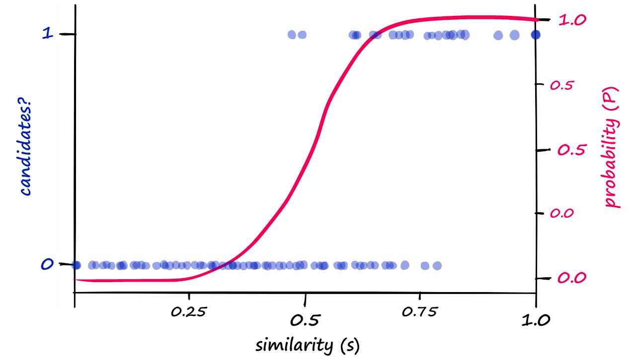

LSH S-curve of collision probability vs similarity

The AND-OR structure turns collision probability into an S-curve in similarity — a phase transition. Source: CS336 Lecture 14.

Tuning the phase transition

Increasing r (hashes per band) sharpens and moves the threshold right (harder to match); increasing b (bands) moves it left (easier). The transition sits at ≈ (1/b)^(1/r), where collision probability is the constant 1 − (1−1/b)^b ≈ 1−1/e ≈ 0.64. A real setting: n=9000, b=20, r=450. This is MinHash-LSH — and dedup should be done across all datasets, not just within each.

From vibes to regression

A model trains on many sources (Wikipedia, web, code, math…); the mixture is a distribution over them. Baselines: vibes (manual — surprisingly common), uniform, and proportional (∝ tokens, but a huge low-quality source dominates). You want to upweight quality but ensure diversity (incomparable sources) and respect that each source is finite:

low = 10T tokens (abundant),  high = 10B tokens (scarce)
mix = {low: 0.5, high: 0.5},  train_tokens = 1T
epochs_on_high = 0.5 · 1T / 10B = 50      # 50× over high-quality data → overfit!

UniMax fixes this with a hard cap on epochs per source. The principled approach is regression-based mixing (RegMix / OLMix): train a swarm of small models on different (e.g. Dirichlet-sampled) mixtures, fit a regression from mixture-weights → loss, optimize it for the best mixture, and scale up — exactly analogous to scaling laws.

⚠️ Two leaps of faith — and the epoching trap

You hope (1) the regression is accurate at its minimizer (you're extrapolating to extremes with little coverage) and (2) the optimal mixture transfers to large scale. And beware overfitting the regression target to downstream evals (lots of code evals → upweight code → bad poetry). The big scale-dependent trap: at small token counts you don't epoch, so the optimizer loves scarce high-quality data — but at large scale that becomes 50× epoching and overfits. Fix with cap epoching or simulated epoching (downsample all sources proportionally so the small run feels the same scarcity). You can also auto-derive domains by a domain × quality grid (Nemotron).

The recipe, and the coding-data arms race

Post-training data is task-dependent and follows one recipe: define environments → define tasks/prompts → collect responses from a strong teacher. In the open community, almost all of it is synthetically generated (a teacher model, sometimes hybrid human-AI). Recent coding datasets show the trajectory:

Dataset	Idea / scale
OpenThoughts	1.2M reasoning examples, QwQ-32B teacher; sampling 16 responses helps; better models aren't better teachers (QwQ-32B > DeepSeek-R1); fewer high-quality sources beat many
SWE-smith	LM generates tasks (introduces bugs) on 128 repos → 50K tasks (semi-synthetic)
SWE-Zero	key observation: strong models solve many SWE tasks without execution feedback → skip the Docker nightmare; 300K trajectories from real PRs; anti-"git-hacking" prompts
SWE-rebench / SWE-Zero-12M	scale to 21K tasks → 12M agent trajectories

The trade-offs

Prompts span fully synthetic → semi-synthetic (real environment + synthetic tasks) → real (actual GitHub PRs). Responses come from capable models that are also good teachers (not the same thing). Code environments are a pain (heavy dependencies, repos that don't run), so a major insight is sidestepping execution entirely — strong models carry an internal "world model" of code semantics. And there's endless filtering and grungy, domain-specific detail.

Golden rules & takeaways

Transform HTML/PDF → text with fast rule-based tools (lossy; the tool choice affects accuracy; PDFs are high-value but expensive).
Filter with the target-vs-raw framework: define what "good" looks like, train a cheap classifier (fastText/KenLM), keep above a threshold. There's no universal threshold — it depends on your token budget.
Deduplicate with hashing for linear-time scale: exact (group by hash), near-dup via MinHash (collision ≈ Jaccard) + LSH bands (AND-OR → sharp S-curve threshold). Dedup across all datasets, not just within.
Mix sources with regression-based mixing (small-scale swarm → fit → optimize → scale up), but cap or simulate epoching so you don't overfit scarce high-quality sources.
Post-training data is mostly synthetic — environments + tasks + a strong (and good) teacher; the coding-data frontier is scaling agent trajectories, sometimes without execution.
Data work is grungy and domain-specific — you have to look at concrete examples; much of the pipeline is still heuristic, with lots of room to improve.

Next: alignment — turning a base model into a helpful, aligned assistant (SFT, preference optimization, RL).

References

Primary source is the lecture (executable lecture_14.py). Key works:

The data pipeline — and synthetic post-training data