Why inference matters more than ever

Inference is everywhere: chatbots, code completion, agents, batch data processing, evaluation, and RL rollouts. And unlike training (a one-time cost), it's a repeated cost. OpenAI is estimated to produce ~8.6 trillion tokens/day; DeepSeek-V4 was trained on ~32T tokens — so in under four days OpenAI's inference compute exceeds a full pre-training run. The agentic shift makes it starker: a query triggers a long internal trace (think, call tools, introspect) before any human-readable output, so tokens generated = compute spent, with no upper bound. A 10% inference speedup is a big deal.

Popular open-source servers: vLLM (PagedAttention, good default), SGLang (agentic workloads), TensorRT-LLM (NVIDIA, fast/narrow), llama.cpp (CPU/local).

Arithmetic-intensity refresher

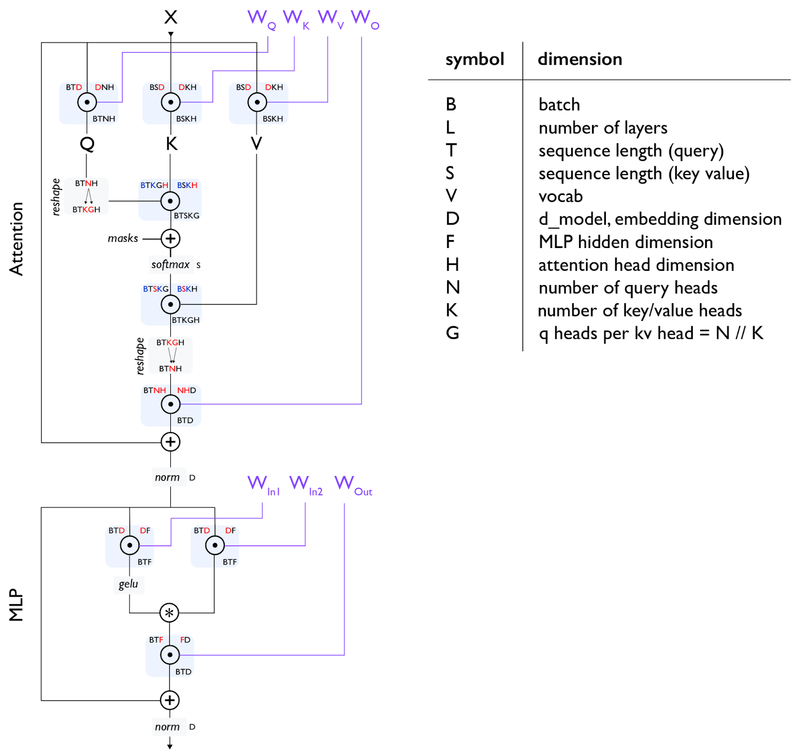The transformer block as a precise tensor diagram — shapes and dependencies made explicit. Notation: F=4D, D=N·H, N=K·G (GQA), S=T in training. Source: "How to Scale Your Model".

For a matmul X[B×D] @ W[D×F] in bf16:

FLOPs   = 2·B·D·F
bytes   = 2·B·D + 2·D·F + 2·B·F        # read X, read W, write Y
intensity = FLOPs / bytes  →  B      # when B ≪ D, F

An H100's accelerator intensity is 989e12 / 3.35e12 ≈ 295 FLOPs/byte. So you're compute-bound iff B > 295. The extreme case B=1 (a matrix–vector product) has intensity 1 — deeply memory-bound. That's essentially what generation looks like.

The KV cache, prefill, and generation

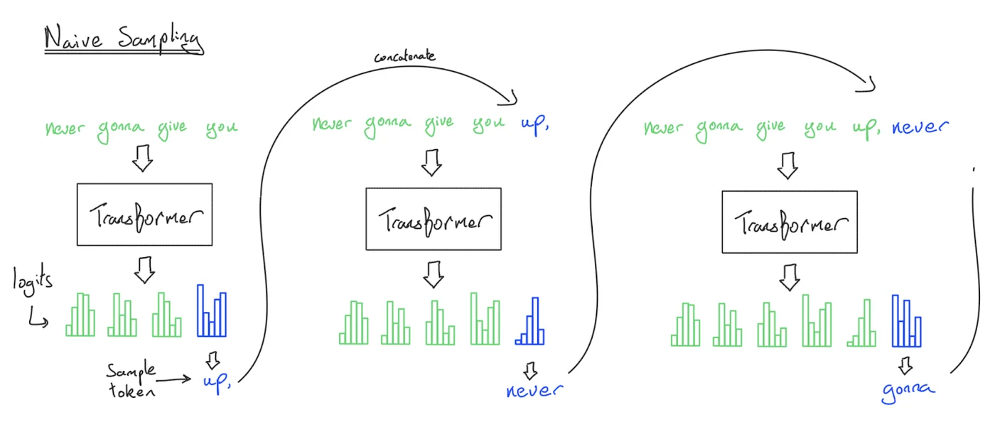Naive generation re-runs the whole sequence each step → generating T tokens costs O(T³). Source: "How to Scale Your Model".

Because the transformer is causal, appended tokens don't change earlier activations — so cache them. The KV cache stores, for every sequence (B), token (S), layer (L), and KV head (K), an H-dimensional key and value, so each step reuses past work.

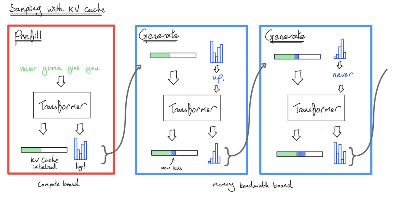Two stages: prefill encodes the prompt in parallel (like training); generation emits tokens sequentially, reusing the cache. Source: "How to Scale Your Model".

Counting FLOPs vs bytes for each layer (S = tokens conditioned on, T = tokens generated):

# MLP (3 matmuls): intensity → B·T   (when B·T ≪ D,F)
# Attention (FlashAttention): intensity → S·T / (S+T)

Latency vs throughput

Since inference is memory-bound (assuming compute/comms overlap), latency = memory ÷ bandwidth. Memory is parameters plus a KV cache that grows with batch:

kv_cache_per_seq = S · (K·H) · L · 2 · 2     # ×2 key+value, ×2 bf16
memory   = B · kv_cache_per_seq + 2·params
latency  = memory / memory_bandwidth          # linear in B
throughput = B / latency                       # rises, then asymptotes

For Llama 2 13B on an H100:

Lower-dimensional KV caches

Memory is the bottleneck and the KV cache can exceed the parameters at large batch — so shrink it, carefully.

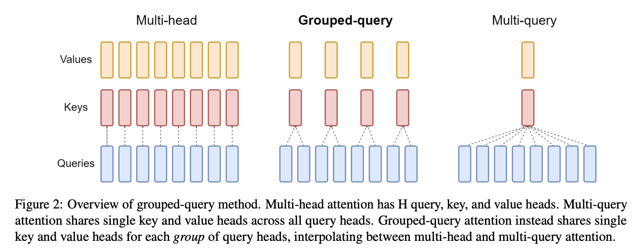MHA (K=N) → GQA (K groups of query heads share K/V) → MQA (K=1). GQA cuts the KV cache by N/K with little accuracy loss. Source: "How to Scale Your Model".

GQA — grouped-query attention

N query heads but only K key/value heads → KV cache ÷ (N/K). MHA (K=N) is full; MQA (K=1) is fastest but "nobody uses it, it's bad"; GQA sits in between. On Llama 2 13B, dropping K 40→8 frees enough memory to also raise the batch (so latency and throughput both improve).

MLA — multi-head latent attention (DeepSeek)

Keep K/V per token but compress them: store a small latent c = W_c·h (DeepSeek-V2: 16384 → 512 dims), project up to K, V on demand. Wrinkle: incompatible with RoPE, so add ~64 RoPE dims (512+64=576). DeepSeek reports MLA ≥ MHA accuracy at far lower cost — and that GQA actually does lose some accuracy (in tension with the GQA paper — take single-model accuracy claims with a grain of salt).

CLA — cross-layer attention

Share K/V across layers (compute KV for a subset, reuse for the rest) — as GQA shares across heads. Improves the accuracy↔KV-cache Pareto frontier.

Local attention & sparse variants

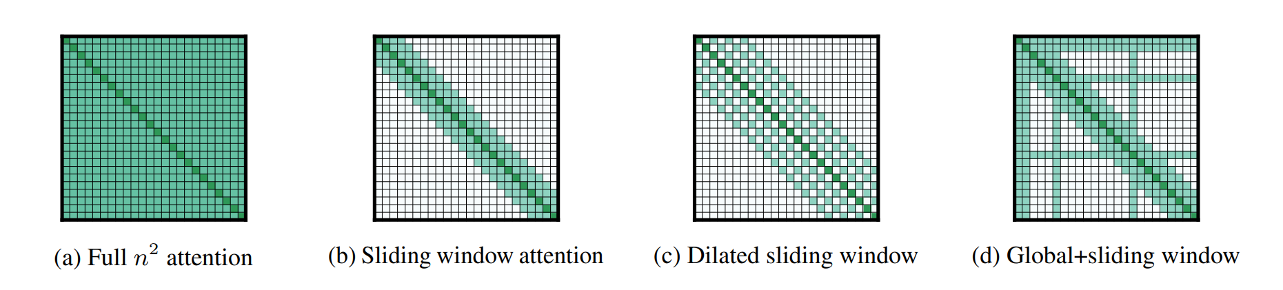Sliding-window attention: each token attends to the last K → KV cache becomes independent of sequence length; effective context grows with depth. Source: CS336 Lecture 10 / Longformer.

Local/sliding-window attention truncates the cache (great for long context), but reduces expressivity and hurts accuracy — so the fix is hybrid layers: interleave a few global-attention layers with many local ones. DeepSeek-V4 (1M context) stacks CSA (compress every m tokens), DSA (select top-k via a lightweight index), and HCA (compress more). Linear-attention / SSMs (Mamba-2, gated DeltaNet) and diffusion are alternatives that compress history into a fixed state.

Quantization & pruning

Quantization reduces numeric precision (bf16 → fp8 → int8 → int4): less memory → higher latency/throughput. Quantize/dequantize via a scale and zero-point. Quantization-aware training simulates quantization in the forward pass (robust, but needs expensive training); post-training quantization is cheaper — GPTQ uses Hessian info to correct quantization error layer-by-layer; AWQ keeps the 0.1–1% of weights tied to large activation channels in high precision (fp16→int3: ~4× less memory, ~3.2× speedup).

Pruning + distillation (NVIDIA Minitron): on a small calibration set, rank the importance of layers/heads/hidden units (by activation magnitude/variance), rip out the unimportant ones, then distill the original model into the pruned one to heal it — e.g. 15B → 8B with little accuracy loss and far less compute than training from scratch.

Exploit "checking is faster than generating"

Prefill verifies many tokens in parallel (compute-bound); generation is one-at-a-time (memory-bound). So use a cheap draft model p to guess k tokens, then have the expensive target model q score all k in one parallel pass and accept/reject:

for each draft token (sampled from p):
    accept with probability  min(1, q/p)        # oversampled by draft → likely reject
    else: sample from the residual  max(q − p, 0)  and stop

This is modified rejection sampling — and the key property is that it produces an exact sample from the target model (provably: P[sampling A] works out to q(A)). You get bursts of accepted tokens. Too few draft tokens wastes the target's parallelism; too many means more rejections — the sweet spot is ~3–4. The draft model should be small but close to the target (so people distill it — the same toolbox as above). Extensions: Medusa (draft generates several tokens in parallel) and EAGLE (draft reuses the target's features).

Continuous & selective batching

Live requests arrive at different times, share prefixes, and have different lengths — far from training's neat dense blocks. Continuous batching (Orca) does iteration-level scheduling: decode one token for all active sequences each step, evict finished ones, and add new arrivals into the batch immediately (no waiting for the whole batch to finish).

But batching needs uniform shapes, and requests have different lengths. Selective batching handles this: process attention per-sequence (it depends on each sequence's length), but concatenate all sequences for the MLP layers (which dominate FLOPs) into one "mega-sequence" — e.g. lengths 3, 9, 5 → a single [17, H] tensor.

PagedAttention (vLLM)

How is the KV cache stored in memory? Naively you pre-allocate a contiguous block per request up to the max length — causing internal fragmentation (most of the reserved space goes unused) and external fragmentation (unusable gaps between requests), exactly like an un-defragmented hard drive.

The fix borrows from operating systems: divide each sequence's KV cache into fixed-size, non-contiguous blocks with an index table. Then sequences can share blocks — cache a shared system prompt once for all queries, or share a prompt's cache across multiple sampled responses — using copy-on-write at the block level (split a block only when generations diverge). Plus fused block-read+attention kernels, FlashAttention/FlashDecoding, and CUDA graphs to cut launch overhead.

Golden rules & takeaways

• Inference is memory-bound because generation is autoregressive — prefill is compute-bound (good), but generation-attention intensity is <1 and can't be improved within a transformer.
• Latency vs throughput is a batch-size trade-off: small batch = low latency, large batch = high throughput (until you hit memory). TTFT ≈ prefill time.
• The KV cache is the lever. Shrink it — GQA (across heads), MLA (compression), CLA (across layers), local/sparse attention (truncation) — without hurting accuracy.
• Quantize, prune, distill to make the model itself cheaper.
• Speculative sampling is lossless: a cheap draft proposes, the target verifies in parallel, and you still get exact target samples.
• Borrow from systems for live traffic: continuous + selective batching, and PagedAttention's OS-style paging and prefix sharing.
• New architectures are the big opportunity — the KV cache makes the transformer inherently inference-unfriendly; an architecture designed for inference (SSMs, linear attention, diffusion) could unlock a lot.

Next: Tatsu returns for Scaling Laws, Part 2 (advanced — μP and optimizers).

References

Primary source is the lecture (executable lecture_10.py) and the "How to Scale Your Model" inference chapter. Key works:

1. How To Scale Your Model — inference chapter
2. Ainslie et al. (2023) — GQA
3. DeepSeek-V2 (2024) — Multi-head Latent Attention
4. Brandon et al. (2024) — Cross-Layer Attention
5. Beltagy et al. (2020) — Longformer (local attention)
6. Frantar et al. (2022) — GPTQ · Lin et al. (2023) — AWQ
7. Muralidharan et al. (2024) — Minitron (pruning + distillation)
8. Leviathan et al. (2022) · Chen et al. (2023) — speculative decoding
9. Medusa · EAGLE
10. Yu et al. (2022) — Orca (continuous batching) · Kwon et al. (2023) — vLLM / PagedAttention